Formula to return a number based on the content of another cell

[canarycat123]

Hi there, I’m hoping someone can help me with this question.

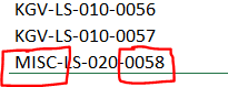
I have a series of formula being used to generate unique reference numbers, finishing with CONCATENATE, as seen in the screencap attached. I am using a simple =IF(H60=””,””,ROW()-2) formula to generate the final four digits of the reference number. However, what I am trying to achieve is slightly more complex.

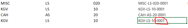
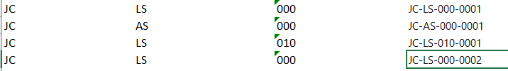
The first portion of characters, in this example KGV and MISC (produced in another cell using VLOOKUP), represent different geographical areas. What I would like to achieve is a formula that can identify the next number in the series related to each geographical area. So, in the attached example I would like MISC to return MISC-LS-020-001 (rather than -0058), as that would be the first KGV record in the worksheet. If I were then to add another MISC I want it to return 002 and so on. If I were then to add another KGV record it should start with the next number in the sequence related to KGV, 0058 in this example.

Any help/advice would be appreciated!

 

[Fluff]

Can you post some sample data.

MrExcel has a tool called “XL2BB” that lets you post samples of your data that will allow us to copy/paste it to our Excel spreadsheets, so we can work with the same copy of data that you are. Instructions on using this tool can be found here: XL2BB Add-in

Note that there is also a "Test Here” forum on this board. This is a place where you can test using this tool (or any other posting techniques that you want to test) before trying to use those tools in your actual posts.

 

[canarycat123]

Can you post some sample data.

MrExcel has a tool called “XL2BB” that lets you post samples of your data that will allow us to copy/paste it to our Excel spreadsheets, so we can work with the same copy of data that you are. Instructions on using this tool can be found here: XL2BB Add-in

Note that there is also a "Test Here” forum on this board. This is a place where you can test using this tool (or any other posting techniques that you want to test) before trying to use those tools in your actual posts.

Hi there, unfortunately my employers doesn't allow 3rd party add-ons.

 

[Fluff]

In that case can you just copy/paste some sample data to the board.

 

[canarycat123]

Does this help?

Formula's for each column are as follows:

Column A: =VLOOKUP(Hxx,Building,2,FALSE)
Column B: =VLOOKUP(Hxx,Location,2,FALSE)
Column C: =VLOOKUP(Hxx,Level,2,FALSE)
Column D: =ROW()-2
Column E: =CONCATENATE(Axx,"-",Bxx,"-",Cxx,"-","00",Dxx)

KGV	LS	010	52​	KGV-LS-010-0052
KGV	LS	010	53​	KGV-LS-010-0053
KGV	LS	010	54​	KGV-LS-010-0054
KGV	LS	010	55​	KGV-LS-010-0055
KGV	LS	010	56​	KGV-LS-010-0056
KGV	LS	010	57​	KGV-LS-010-0057
MISC	LS	020	58​	MISC-LS-020-0058

 

[Fluff]

Thanks for that, how about

+Fluff 1.xlsm
	A	B	C	D	E
1
2	KGV	LS	10	52	KGV-LS-10-0001
3	KGV	LS	10	53	KGV-LS-10-0002
4	KGV	LS	10	54	KGV-LS-10-0003
5	KGV	LS	10	55	KGV-LS-10-0004
6	KGV	LS	10	56	KGV-LS-10-0005
7	KGV	LS	10	57	KGV-LS-10-0006
8	MISC	LS	20	58	MISC-LS-20-0001
Test

Cell Formulas
Range	Formula
E2:E8	E2	=TEXTJOIN("-",,A2:C2,TEXT(COUNTIFS(E$1:E1,A2&"-"&B2&"-"&C2&"-*")+1,"0000"))

 

[canarycat123]

Thanks for that, how about

+Fluff 1.xlsm
	A	B	C	D	E
1
2	KGV	LS	10	52	KGV-LS-10-0001
3	KGV	LS	10	53	KGV-LS-10-0002
4	KGV	LS	10	54	KGV-LS-10-0003
5	KGV	LS	10	55	KGV-LS-10-0004
6	KGV	LS	10	56	KGV-LS-10-0005
7	KGV	LS	10	57	KGV-LS-10-0006
8	MISC	LS	20	58	MISC-LS-20-0001
Test

Cell Formulas
Range	Formula
E2:E8	E2	=TEXTJOIN("-",,A2:C2,TEXT(COUNTIFS(E$1:E1,A2&"-"&B2&"-"&C2&"-*")+1,"0000"))

Brilliant! I'd day we're 80% there. In the attached example, because there are now 2 KGV records the final portion of the ref should be 002. Is that possible?

 

[Fluff]

It should give you that, as can be seen in post#6

 

[canarycat123]

It should give you that, as can be seen in post#6

Ah yes, I made a tweak and now it works. The last thing to overcome is a follows, hopefully there's a way of doing this: The last four digits of the ref should be based only on the location (first element of the ref). In the attached example, the four digit ref is starting from 0001 when the second and third elements form a unique combination. In the attached example, even though the second and third elements are different, because the first portion is 'JC' it should number from 0001-0004 consecutively. Does that make sense?

 

[Fluff]

Do you mean that the last 4 numbers should increment solely based on the value in col A?