Fuel Mileage Calculation

[guamlenahans]

Hi,
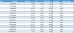
I have a table where i track fuel purchased for 7 vehicles. Vehicles are tracked by plate number. My columns are: Date, Vehicle, Gallons, Cost, Total Cost, and odometer. We enter them row after row and I pivot out the gallons for each vehicle. I'm trying to add two columns where I will factor in the miles driven and the miles per gallon. I will need the formula to look back at the last entry for the vehicle and calculate the miles driven between then and the latest fill up based on the odometer readings. I cant figure out how to do that.

Ideas?

Thanks

Rob

 

[jasonb75]

Based on how yuo desscribe your sheet, I would suggest using vlookup to get the odometer difference, assuming that your table fills columns A:G, with headers in row 1, in H2 enter and fill down

=IFERROR(F2-VLOOKUP(B2,B$1:F1,5,0),"")

Then in I2 and fill down for the MPG

=IF(H2="","",C2/H2)

 

[guamlenahans]

Thanks Jason. tried it but not working. My sheet look like this:

 

[AhoyNC]

What version of Excel are you using?

 

[guamlenahans]

2016

 

[jasonb75]

The second formula is wrong, I miscounted the columns and had the division in reverse, it should be this in H2

=IF(G2="","",G2/C2)

The first formula is correct, but it needs to go into G2 instead of H2 before filling down.

 

[guamlenahans]

The first formula not returning any value?

 

[jasonb75]

The first row for each vehicle will be blank as there is no history, but after you fill it down the subsequent rows should show results.

edit:- looking at your screen capture, the first result should be row 7.

 

[AhoyNC]

Here is another option that seems to work for mileage. If there is not a previous record it just returns odometer reading.

Book1
	A	B	C	D	E	F	G
1	Date	Vehicle	Gallons	Cost	Total	Odometer	Miles
2	7/1/2019	Veh1				43000	43000
3	7/3/2019	Veh2				20000	20000
4	7/3/2019	Veh3				56000	56000
5	7/1/2019	Veh4				35000	35000
6	7/8/2019	Veh1				43275	275
7	7/17/2019	Veh6				10000	10000
8	7/18/2019	Veh7				89500	89500
9	7/24/2019	Veh8				35600	35600
10	7/25/2019	Veh2				20400	400
11	8/6/2019	Veh1				43915	640
12	8/13/2019	Veh3				56388	388
13	8/14/2019	Veh7				89832	332
14	8/19/2019	Veh1				44156	241
Sheet1

Cell Formulas
Range	Formula
G2:G14	G2	=F2-IFERROR(INDEX($F$2:F2,AGGREGATE(14,6,(ROW($F$2:F2)-ROW($F$2)+1)/($B$2:B2=B2),2)),0)

 

[guamlenahans]

Agree. I have this in cell 7, not getting any result: