Get a row value from a Pivot Table.

[admat]

Hello all,

I had this formula to return the first 5 Rows of a Table:

INDEX(SUMMARY[EMPNAME],D2,1)
INDEX(SUMMARY[EMPNAME],D2+1,1)
INDEX(SUMMARY[EMPNAME],D2+2,1)
INDEX(SUMMARY[EMPNAME],D2+3,1)
INDEX(SUMMARY[EMPNAME],D2+4,1)

I enter 1 in D2 and it returns the first 5 rows. Change it to 6 and it will show the next 5 rows.

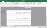
I now that I have the data in a Pivot Table. How do I reference the rows to accomplish the same thing?

I am trying to get the Pivot Table data in a fixed template for printing.

 

[Anthony47]

I don't know if you can get it via formulas, but you can do that via a User Defined Function, with a lot of flexibility.
For example, insert the following code into a "standard module" of your vba project:

 Function PVT_Rows(ByRef PVTab As Range, ByVal iRow As Long, ByVal RNum As Long, Optional ByVal CNum As Long = 0, Optional ByVal RHYN As Boolean = True) As Variant
'https://www.mrexcel.com/board/threads/get-a-row-value-from-a-pivot-table.1126731/
'
'Returns N rows from a PivotTable
'USE: ==============================================================
'   =PVT_Rows(Address of any cell in the target PivotTable,StartingRow, HowManyRows, [optional: HowManyColumn, [optional: RowHeadingsYes]])
'
'example
'   =PVT_Table(Sheet3!A4,1,3)         'shall return lines 1-2-3 from PvtTable in Sheet3!A4
'   =PVT_Table(Sheet3!A4,2,3,4)       'shall return lines 2-3-4, columns HR+1-2-3-4 from PvtTable in Sheet3.A4
'   =PVT_Table(Sheet3!A4,1,3,,False)  'shall return lines 1-2-3 from PvtTable in Sheet3!A4, without RowHeaders
'
'   NB: HR means all the Field Names on the row
'       iRow can be 0, that corresponds to the column headers
'===================================================================
Dim pSheet As Worksheet, rHead As Long, oArr
Dim pCC As Long, pRC As Long
'
Set pSheet = PVTab.Parent
'
PV1 = PVTab.PivotTable.Name
If RHYN Then rHead = pSheet.PivotTables(PV1).RowRange.Columns.Count
pCC = pSheet.PivotTables(PV1).DataBodyRange.Columns.Count
pRC = pSheet.PivotTables(PV1).DataBodyRange.Rows.Count
If CNum = 0 Or CNum > pCC Then CNum = pCC
If iRow < 0 Then iRow = 0
If (iRow + RNum) > pRC Then
    If iRow > pRC Then iRow = pRC
    RNum = pRC - iRow + 1
    If RNum < 1 Then
        RNum = 1
        iRow = 0
    End If
End If
oArr = pSheet.PivotTables(PV1).DataBodyRange.Cells(iRow, 1).Offset(0, -rHead).Resize(RNum, CNum + rHead).Value
'Cleanup:
For I = 1 To UBound(oArr)
    For j = 1 To rHead
        If oArr(I, j) = 0 Then oArr(I, j) = ""
    Next j
Next I
PVT_Rows = oArr
End Function

Then you will be able to use in your worksheet a formula like

=PVT_Table(Sheet3!A4,1,3)

This will return 3 full lines of the pivot table that take A4 (any cell of the pivotable) in Sheet3, starting from first Row
The formula has to be inserted as an array formula (using Control-Shift-Enter) in the expected number of rows & columns

The syntax for this function:
=PVT_Rows(Address of any cell in the target PivotTable,StartingRow, HowManyRows, [optional: HowManyColumn, [optional: RowHeadingsYes]])

Address of any cell in the target PivotTable: a reference to any cell within the target PivotTable. Ex A4 (cell A4 in the current sheet); Sheet1!A4 (cell A4 in Sheet1)

StartingRow: the first line to start from. StartingRow may be 0, that means "from the headers of the columns"; negative values not allowed

HowManyRows: how many lines to return. If StartingRow + HowManyRows > available rows then these two parametres will be adjusted to return al least the last available row

HowManyColumns: how many columns to return; this is optional, if omitted "All" the columns will be returned. The function will return maximum "All" the columns

RowHeadingsYes: this is optional too; if False, then only the "DataBody" of the table will be returned; if True or omitted then the headers of the rows will also be returned, in addition to the DataBody. Note that this means that by default the function returns more columns than those specified in HowManyColumns

Examples:

   =PVT_Table(Sheet3!A4,1,3)         'shall return lines 1-2-3 from PvtTable in Sheet3!A4
   =PVT_Table(Sheet3!A4,2,3,4)       'shall return lines 2-3-4, columns HR+1-2-3-4 from PvtTable in Sheet3.A4
   =PVT_Table(Sheet3!A4,1,3,,False)  'shall return lines 1-2-3 from PvtTable in Sheet3!A4, without RowHeaders
   =PVT_Table(Sheet3!A4,1,3000)         'shall return "up to 3000" lines from PvtTable in Sheet3!A4

If you need more instructions or information just ask and "probably" you will get an answer.

Bye

 

[Peter_SSs]

@admat

Could you show us what your pivot table looks like & explain again what you want in relation to that image?

 

[admat]

Ok I think I may have made some headway. on Cell A8 i inserted this formula

=@OFFSET(PTable!$A$4,$B$1-1,0)
A9
=@OFFSET(PTable!$A$4,$B$1,0)
A10
=@OFFSET(PTable!$A$4,$B$1+1,0) and so on.

PTable!$A$4 is the starting cell on my Pivot Table. Everything seems to be working.

 

[Peter_SSs]

That is the sort of way I was headed and why I asked for an image.

However, you should be able to do this
- without using the volatile function OFFSET, and
- without having to do 5 separate formulas.

I suggest that you update your Account details (click your user name at the top right of the forum) so helpers always know what Excel version(s) & platform(s) you are using as the best solution often varies by version.

If you do not have Excel 365 with the SEQUENCE function, try the B2 function copied down.

If you do have the SEQUENCE function then you can just enter the C2 formula and the other results will automatically 'spill' down to the other cells.

20 03 09.xlsm
	B	C
1	3
2	Ken	Ken
3	Ann	Ann
4	Jen	Jen
5	Ted	Ted
6	Joe	Joe
7
Access PT

Cell Formulas
Range	Formula
C2:C6	C2	=INDEX(PTable!A:A,SEQUENCE(5,,B1+3))
B2:B6	B2	=INDEX(PTable!A:A,B$1+ROWS(B$2:B2)+2)
Dynamic array formulas.

Here is part of my pivot table

 

[admat]

Thank you @Peter_SSs , this is a better alternative.

 

[Anthony47]

Had you a chance to test the Function PVT_Rows?

Bye

 

[Peter_SSs]

Thank you @Peter_SSs , this is a better alternative.

You're welcome. .. and thanks for updating your profile.