get table row and column headings based on multiple cells with the same value

[TheColonist]

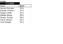
My Table calculates when Progress Reports are due. Those due this week are highlighted in red via conditional formating.
Trying to figure how to list the student name and the report due in one cell on a separate sheet.

Example:
Student 2 PR 5
Student 3 PR 2
Student 5 PR 8
etc.

Many of our instructors are blind, so the current worksheet does not help them. Getting it to list as shown above would allow it to be copied and pasted in an email to alert everyone what reports are do.
I work for a state agency and we are not allowed to use Macros, so no VB code.
Using Office 365 on Windows 10

 

[KRice]

Here is one approach. Note that I first create a list of students meeting the date criterion anywhere on their row, then the specific reports are listed beside their name. To illustrate what happens should multiple reports be due for one student, I changed the yellow cell from 7/21/2023 to a date that fell within the week given in cell N1 (so that two reports are due for Student 2).

Staffing Schedule Calculator.xlsx
	A	B	C	D	E	F	G	H	I	J	K	L	M	N
1													Week beginning:	6/18/2023
2
3	Student	Program	Assessment Begins	Staffing ICP	Training Begins	PR 1	PR 2	PR 3	PR 4	PR 5	PR 6		Reports Due:
4	Student 1	VISP	1/9/2023	1/20/2023	1/23/2023	2/17/2023	3/17/2023	4/14/2023	5/12/2023	6/9/2023	7/7/2023		Student 2	PR 5, PR 6
5	Student 2	VISP	1/23/2023	2/3/2023	2/6/2023	3/3/2023	3/31/2023	4/28/2023	5/26/2023	6/23/2023	6/23/2023		Student 3	PR 2
6	Student 3	VISP	4/17/2023	4/28/2023	5/1/2023	5/26/2023	6/23/2023	7/21/2023	8/18/2023	9/15/2023	10/13/2023		Student 10	Staffing ICP
7	Student 4	VISP	3/6/2023	3/17/2023	3/20/2023	4/14/2023	5/12/2023	6/9/2023	7/7/2023	8/4/2023	9/1/2023		Student 15	Staffing ICP
8	Student 5	AT	10/31/2022	11/11/2022	11/14/2022	12/9/2022	1/6/2023	2/3/2023	3/3/2023	3/31/2023	4/28/2023		Student 18	PR 1
9	Student 6	AT	7/11/2022	7/22/2022	7/25/2022	8/19/2022	9/16/2022	10/14/2022	11/11/2022	12/9/2022	1/6/2023
10	Student 7	AT	4/4/2022	4/15/2022	4/18/2022	5/13/2022	6/10/2022	7/8/2022	8/5/2022	9/2/2022	9/30/2022
11	Student 8	VISP	4/3/2023	4/14/2023	4/17/2023	5/12/2023	6/9/2023	7/7/2023	8/4/2023	9/1/2023	9/29/2023
12	Student 9	VISP	6/2/2023	6/13/2023	6/16/2023	7/13/2023	8/10/2023	9/7/2023	10/5/2023	11/2/2023	12/7/2023
13	Student 10	VISP	6/12/2023	6/23/2023	6/26/2023	7/21/2023	8/18/2023	9/15/2023	10/13/2023	11/10/2023	12/15/2023
14	Student 11	VISP	8/8/2022	8/19/2022	8/22/2022	9/16/2022	10/14/2022	11/11/2022	12/9/2022	1/6/2023	2/3/2023
15	Student 12	VISP	8/8/2022	8/19/2022	8/22/2022	9/16/2022	10/14/2022	11/11/2022	12/9/2022	1/6/2023	2/3/2023
16	Student 13	AT	10/3/2022	10/14/2022	10/17/2022	11/11/2022	12/9/2022	1/6/2023	2/3/2023	3/3/2023	3/31/2023
17	Student 14	VISP	1/9/2023	1/20/2023	1/23/2023	2/17/2023	3/17/2023	4/14/2023	5/12/2023	6/9/2023	7/7/2023
18	Student 15	VISP	6/12/2023	6/23/2023	6/26/2023	7/21/2023	8/18/2023	9/15/2023	10/13/2023	11/10/2023	12/15/2023
19	Student 16	AT	10/13/2022	10/24/2022	10/27/2022	11/23/2022	12/21/2022	1/18/2023	2/15/2023	3/15/2023	4/12/2023
20	Student 17	VISP	10/17/2022	10/28/2022	10/31/2022	11/25/2022	12/23/2022	1/20/2023	2/17/2023	3/17/2023	4/14/2023
21	Student 18	VISP	5/15/2023	5/26/2023	5/29/2023	6/23/2023	7/21/2023	8/18/2023	9/15/2023	10/13/2023	11/10/2023
22	Student 19	VISP	4/3/2023	4/14/2023	4/17/2023	5/12/2023	6/9/2023	7/7/2023	8/4/2023	9/1/2023	9/29/2023
23	Student 20	VISP	5/1/2023	5/12/2023	5/15/2023	6/9/2023	7/7/2023	8/4/2023	9/1/2023	9/29/2023	10/27/2023
24	Student 21	VISP	5/30/2023	6/10/2023	6/13/2023	7/10/2023	8/7/2023	9/4/2023	10/2/2023	10/30/2023	12/4/2023
Sheet1

Cell Formulas
Range	Formula
M4:M8	M4	=FILTER($A$4:$A$24,BYROW(($C$4:$K$24-$N$1<=6)*($C$4:$K$24-$N$1>=0),LAMBDA(x,SUM(x)))>0)
N4:N8	N4	=TEXTJOIN(", ",TRUE,FILTER($C$3:$K$3,FILTER(($C$4:$K$24-$N$1<=6)*($C$4:$K$24-$N$1>=0),$A$4:$A$24=M4)=1))
Dynamic array formulas.

 

[TheColonist]

Fantastic! New to the Filter function, but love it. I figured the N4 formula would contain nested Filters. Had to familiarize myself with LAMBDA and BYROW.
Thanks for the help!

 

[TheColonist]

Well, thought I understood. Not sure what the LAMBDA(x,SUM(x)) is doing.

 

[KRice]

Glad to help. The ($C$4:$K$24-$N$1<=6)*($C$4:$K$24-$N$1>=0) part of the formula creates an array that mirrors the data table in $C$4:$K$24, except each entry assumes the value of either 1 or 0 to indicate whether the entry is within the next six days of the "week beginning" date in $N$1. The 1's and 0's are formed because the TRUEs and FALSEs returned by the logical checks are coerced to 1's and 0's when the arrays are multiplied together. We'll use this two-dimensional array of 1's and 0's to determine which rows have at least one "1" in them...those are the rows of interest.

The BYROW function accepts a LAMBDA function as one of it's arguments. So we feed the two-dimensional array of 1's and 0's to the BYROW function, and BYROW takes one row at a time and feeds it to the LAMBDA function (so each row is treated as "x" in the LAMBDA function), and then that x (that row) is summed (the SUM(x) component in the LAMBDA function). So if you have two reports due within the next week for a given student, this expression will evaluate to 2 (i.e., if we were to look across this row in the two-dimensional array of 1's and 0's, we would find two 1's corresponding to dates that are within the next 6 days of the "week beginning" date in $N$1). We care about identifying any rows where this sum is >0, which is the criteria used by FILTER for trimming down the list of students in $A$4:$A$24.

The "old school" approach to summing across each row involves some linear algebra using the MMULT function. Here is a comparison of the two, operating on the two dimensional array of 1's and 0's:

Staffing Schedule Calculator.xlsx
	Q	R	S	T	U	V	W	X	Y	Z	AA	AB	AC
3		AB	SICP	TB	PR1	PR2	PR3	PR4	PR5	PR6
4	Student 1	0	0	0	0	0	0	0	0	0		0	0
5	Student 2	0	0	0	0	0	0	0	1	1		2	2
6	Student 3	0	0	0	0	1	0	0	0	0		1	1
7	Student 4	0	0	0	0	0	0	0	0	0		0	0
8	Student 5	0	0	0	0	0	0	0	0	0		0	0
9	Student 6	0	0	0	0	0	0	0	0	0		0	0
10	Student 7	0	0	0	0	0	0	0	0	0		0	0
11	Student 8	0	0	0	0	0	0	0	0	0		0	0
12	Student 9	0	0	0	0	0	0	0	0	0		0	0
13	Student 10	0	1	0	0	0	0	0	0	0		1	1
14	Student 11	0	0	0	0	0	0	0	0	0		0	0
15	Student 12	0	0	0	0	0	0	0	0	0		0	0
16	Student 13	0	0	0	0	0	0	0	0	0		0	0
17	Student 14	0	0	0	0	0	0	0	0	0		0	0
18	Student 15	0	1	0	0	0	0	0	0	0		1	1
19	Student 16	0	0	0	0	0	0	0	0	0		0	0
20	Student 17	0	0	0	0	0	0	0	0	0		0	0
21	Student 18	0	0	0	1	0	0	0	0	0		1	1
22	Student 19	0	0	0	0	0	0	0	0	0		0	0
23	Student 20	0	0	0	0	0	0	0	0	0		0	0
24	Student 21	0	0	0	0	0	0	0	0	0		0	0
Sheet1

Cell Formulas
Range	Formula
R4:Z24	R4	=(C4:K24-$N$1<=6)*(C4:K24-$N$1>=0)
AB4:AB24	AB4	=BYROW(R4#,LAMBDA(x,SUM(x)))
AC4:AC24	AC4	=MMULT($R$4:$Z$24,TRANSPOSE(COLUMN(R3:Z3)^0))
Q4:Q24	Q4	=A4
Dynamic array formulas.

 

[TheColonist]

I got the output I wanted before I posted, but hoped for more compact formulas, like what you did. Here is what I came up with:

For the Student name: (messy, but it works)

=FILTER(Table1[Student],
(Table1[Staffing ICP]=$A$2)+
(Table1[PR 1]=$A$2)+
(Table1[PR 2]=$A$2)+
(Table1[PR 3]=$A$2)+
(Table1[PR 4]=$A$2)+
(Table1[PR 5]=$A$2)+
(Table1[PR 6]=$A$2),"")

For the Report Due: (got this from a YouTube video)

=IF(A4="","",INDEX(Table1[[#Headers],[Staffing ICP]:[PR 10]],,
MATCH($A$2,INDEX(Table1[[Staffing ICP]:[PR 10]],
MATCH(A4,Table1[Student],0),),0)))

I like yours and will play with it to make it work for me.
Thanks for your help KRice

 

[KRice]

Here is a version that uses a formal named table (Table1) as suggested in your last post. Will there every be occasions where more than one report is due for a given student...as I've shown for Student 2 in this example? I ask because the MATCH function you've described will find only the first match, but not all of them if there are multiple reports for a student.

Staffing Schedule Calculator.xlsx
	A	B	C	D	E	F	G	H	I	J	K	L	M	N
1													Due Week of:
2													6/18/2023
3	Student	Program	Assessment Begins	Staffing ICP	Training Begins	PR 1	PR 2	PR 3	PR 4	PR 5	PR 6		Student	Report
4	Student 1	VISP	1/9/2023	1/20/2023	1/23/2023	2/17/2023	3/17/2023	4/14/2023	5/12/2023	6/9/2023	7/7/2023		Student 2	PR 5, PR 6
5	Student 2	VISP	1/23/2023	2/3/2023	2/6/2023	3/3/2023	3/31/2023	4/28/2023	5/26/2023	6/23/2023	6/23/2023		Student 3	PR 2
6	Student 3	VISP	4/17/2023	4/28/2023	5/1/2023	5/26/2023	6/23/2023	7/21/2023	8/18/2023	9/15/2023	10/13/2023		Student 10	Staffing ICP
7	Student 4	VISP	3/6/2023	3/17/2023	3/20/2023	4/14/2023	5/12/2023	6/9/2023	7/7/2023	8/4/2023	9/1/2023		Student 15	Staffing ICP
8	Student 5	AT	10/31/2022	11/11/2022	11/14/2022	12/9/2022	1/6/2023	2/3/2023	3/3/2023	3/31/2023	4/28/2023		Student 18	PR 1
9	Student 6	AT	7/11/2022	7/22/2022	7/25/2022	8/19/2022	9/16/2022	10/14/2022	11/11/2022	12/9/2022	1/6/2023
10	Student 7	AT	4/4/2022	4/15/2022	4/18/2022	5/13/2022	6/10/2022	7/8/2022	8/5/2022	9/2/2022	9/30/2022
11	Student 8	VISP	4/3/2023	4/14/2023	4/17/2023	5/12/2023	6/9/2023	7/7/2023	8/4/2023	9/1/2023	9/29/2023
12	Student 9	VISP	6/2/2023	6/13/2023	6/16/2023	7/13/2023	8/10/2023	9/7/2023	10/5/2023	11/2/2023	12/7/2023
13	Student 10	VISP	6/12/2023	6/23/2023	6/26/2023	7/21/2023	8/18/2023	9/15/2023	10/13/2023	11/10/2023	12/15/2023
14	Student 11	VISP	8/8/2022	8/19/2022	8/22/2022	9/16/2022	10/14/2022	11/11/2022	12/9/2022	1/6/2023	2/3/2023
15	Student 12	VISP	8/8/2022	8/19/2022	8/22/2022	9/16/2022	10/14/2022	11/11/2022	12/9/2022	1/6/2023	2/3/2023
16	Student 13	AT	10/3/2022	10/14/2022	10/17/2022	11/11/2022	12/9/2022	1/6/2023	2/3/2023	3/3/2023	3/31/2023
17	Student 14	VISP	1/9/2023	1/20/2023	1/23/2023	2/17/2023	3/17/2023	4/14/2023	5/12/2023	6/9/2023	7/7/2023
18	Student 15	VISP	6/12/2023	6/23/2023	6/26/2023	7/21/2023	8/18/2023	9/15/2023	10/13/2023	11/10/2023	12/15/2023
19	Student 16	AT	10/13/2022	10/24/2022	10/27/2022	11/23/2022	12/21/2022	1/18/2023	2/15/2023	3/15/2023	4/12/2023
20	Student 17	VISP	10/17/2022	10/28/2022	10/31/2022	11/25/2022	12/23/2022	1/20/2023	2/17/2023	3/17/2023	4/14/2023
21	Student 18	VISP	5/15/2023	5/26/2023	5/29/2023	6/23/2023	7/21/2023	8/18/2023	9/15/2023	10/13/2023	11/10/2023
22	Student 19	VISP	4/3/2023	4/14/2023	4/17/2023	5/12/2023	6/9/2023	7/7/2023	8/4/2023	9/1/2023	9/29/2023
23	Student 20	VISP	5/1/2023	5/12/2023	5/15/2023	6/9/2023	7/7/2023	8/4/2023	9/1/2023	9/29/2023	10/27/2023
24	Student 21	VISP	5/30/2023	6/10/2023	6/13/2023	7/10/2023	8/7/2023	9/4/2023	10/2/2023	10/30/2023	12/4/2023
Sheet1

Cell Formulas
Range	Formula
M4:M8	M4	=FILTER(Table1[Student],BYROW((Table1[[Assessment Begins]:[PR 6]]-$M$2<=6)*(Table1[[Assessment Begins]:[PR 6]]-$M$2>=0),LAMBDA(x,SUM(x)))>0)
N4:N8	N4	=TEXTJOIN(", ",TRUE,FILTER(Table1[[#Headers],[Assessment Begins]:[PR 6]],FILTER((Table1[[Assessment Begins]:[PR 6]]-$M$2<=6)*(Table1[[Assessment Begins]:[PR 6]]-$M$2>=0),Table1[Student]=M4)=1))
Dynamic array formulas.