Go to entered date in Excel for Mac 2016

[renpilot]

Hello all experts,

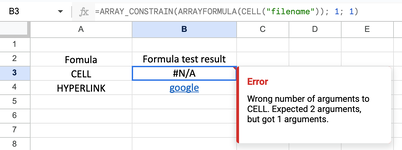
I have tried some VBA solutions I found but they don't work (or maybe I am doing something wrong). I read that Excel for Mac is not as advanced, so maybe that is the reason.

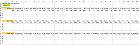
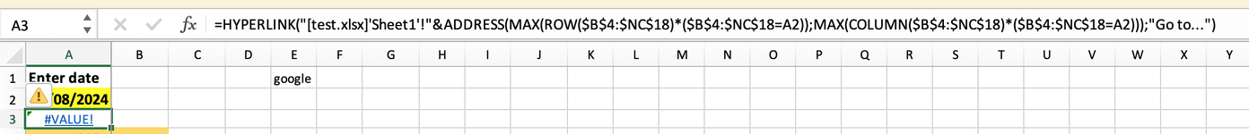
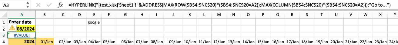
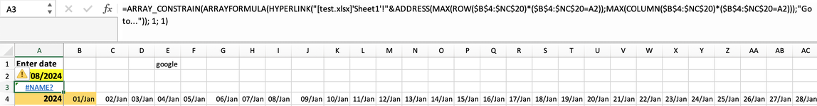
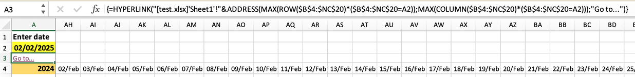
I am trying to make Excel for Mac 2016 go to a date that I enter in A2. The date can be in rows b4:nc4 or b11:nc11 or b18:nc18 as I am displaying the days for three years in these rows. The entered dates in the three rows are dd/mm/yyyy but are displayed as dd/mmm to save space. The entered date is in format dd/mm/yy.

I would like this functionality as it is easier to navigate all these dates when an input has to be made in a cell below the specific date. Column A is frozen so the identifiers will always be visible when scrolling through to any given date.

Hope you have ideas

 

[felixstraube]

Can you upload your test file somewhere for me to download? And post the link here? I will work on it and see what is going on.

As for the CELL function test, your should copy the following text exactly as it is, paste it into any cell and hit enter:

=CELL("filename")

Do not change the text. Do not use the second argument. If it returns an error then it isn't working.

And don't worry about wasting my time. I really want to get to the bottom of this.

 

[renpilot]

=CELL works also.
I have searched a lot online. There seems to be an issue with Excel and the HYPERLINK function, but you are welcome to try.

A link to the test file with your last HYPERLINK formula in cell A3 and your Google HYPERLINK in cell E1 was sent to you as PM, but I don't know if that goes public on the forum...

 

[felixstraube]

So, I detected some problems:
1. In your original post, you attached a image with the year and dates in rows 4, 11 and 18. In your test file these rows are 4, 12 and 20. So the range $B$4:$NC$18 which is used in the formula has to be changed to $B$4:$NC$20 so it will consider the dates of 2026.
2. In your formula you have some "@" in some places and that is what made the formula not work:

=HYPERLINK("[test.xlsx]'Sheet1'!"&ADDRESS(MAX(@ROW($B$4:$NC$18)*(@$B$4:$NC$18=A2)),MAX(@COLUMN($B$4:$NC$18)*(@$B$4:$NC$18=A2))),"Go to...")

The formula should look like this:

=HYPERLINK("[test.xlsx]'Sheet1'!"&ADDRESS(MAX(ROW($B$4:$NC$20)*($B$4:$NC$20=A2)),MAX(COLUMN($B$4:$NC$20)*($B$4:$NC$20=A2))),"Go to...")

Now it should work.

Here I uploaded the corrected file: test.xlsx

I also included a second sheet, named "Sheet2". Can you check what result you get in cell B3 with the CELL formula?

 

[renpilot]

I have no @ in the formula - I have no characters in the positions were you see @. There is just the forward parenthesis and then ROW, $B$4, COLUMN and $B$4. See screenshot 1 of my spreadsheet formula.
With the correct range the HYPELINK formula still returns a #VALUE! error. See screenshot 2
The CELL formula in Sheet2 returns an error. See screenshot 3
I then tried to copy your formula from above and changed the , before MAX and before Go to to a ; - it still returns a #VALUE! error. See screenshot 4
The formula in your spreadsheet is different with an ARRAY. I tried copying that from your test sheet, but it returns a #NAME? error. See screenshot 5.

 

[felixstraube]

Maybe dropbox added the "@"s. Don't know but when I open the file i download from your link there they are.

And I can see from your screenshots that the file I uploaded opened in google sheets and there you got the formulas with the function ARRAYFORMULA() for example.
So I uploaded another file but compressed as ZIP file, this way it wont open in google sheets. Please download it, decompress it and try it out.

Download link: AnotherTest.zip

Can you also go to the sheet "TestSheet" and provide a screenshot of what you see? And try the different hiperlink functions?

Thanks

 

[renpilot]

SO it finally worked. I think it is the fact that you changed the formula to an array with the { } around it.
WHAT seems different in Excel for Mac is to get the array formula you copy and paste the original formula and then press CTRL+SHIFT+ENTER

Thank you so much!
Is there any chance without using VBA to make the curser jump without clicking a hyperlink?
Second best option would be to highligt the cell the hyperlink makes Excel jump to?

 

[renpilot]

=HYPERLINK("[test.xlsx]'Sheet1'!"&ADDRESS(MAX(ROW($B$4:$NC$20)*($B$4:$NC$20=A2));MAX(COLUMN($B$4:$NC$20)*($B$4:$NC$20=A2)));"Go to...")
This formula in CELL A3 worked with CTRL+SHIFT+ENTER

 

[renpilot]

How do I give you credit for the working formula?

 

[felixstraube]

I'm so glad it finally worked.

I don't think that without VBA the jump will be possible.
To highlight the date you could use conditional formatting like so:

I believe you can mark a post as the solution.

And thanks for the feedback.

 

[felixstraube]

Another thing to consider is to organize your data differently. I don't know what you actual data in rows A, B, C, D, E are but you could try this:
To create a table with these columns:

Date	A	B	C	D	E
01/01/2024	10	5	9	3	5
02/01/2024	3	6	8	10	3
03/01/2024	3	7	7	1	7
04/01/2024	5	3	10	2	4
05/01/2024	8	8	5	9	2
06/01/2024	2	1	8	3	2
07/01/2024	6	4	6	6	5
08/01/2024	3	8	1	10	9
09/01/2024	7	8	8	4	3
10/01/2024	4	6	1	3	9
11/01/2024	5	9	1	9	3

With dates from 01/01/2024 to 31/12/2026, and in the A - E columns you data.

Then you could filter the table by date for example

And you'll get this:

You also can do lookups. Enter a date in one cell and get values from columns A to E.

Here is a (hopefully) working example: DataAsTable.zip

Let me know what you think.