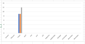
My workbook consists of 12 worksheets. Each worksheet is named for each month of the year. I'd like to add a 13th worksheet that will be the home for the graph(s). Each worksheet is a calendar and looks like a calendar. Let's use March as an example but every worksheet has the same three options. There are 31 days in March. Each one of those days has a drop-down with three options. Let's call them Option 1, Option 2, and Option 3. Let's say that 6 days out of the 31 days were selected as option 1, 10 days out of the 31 were selected as option 2 and 15 days out of the 31 are selected as option 3. What I would like is for my graph located in the 13th worksheet to have 3 bars for each month or one bar showing the 3 options. Each bar will show how many times each option was chosen in that particular month. I'd also like to have a separate graph that totals each option for the year. I appreciate any assistance with this! I have searched and read all kinds of forums and watched Youtube videos but I can't find anything pertaining to what I need.
-
If you would like to post, please check out the MrExcel Message Board FAQ and register here. If you forgot your password, you can reset your password.
You are using an out of date browser. It may not display this or other websites correctly.
You should upgrade or use an alternative browser.
You should upgrade or use an alternative browser.
Greetings everyone! I am having a bit of trouble with adding a graph to my workbook.
- Thread starter KEMPFAT
- Start date
Excel Facts
Which Excel functions can ignore hidden rows?
The SUBTOTAL and AGGREGATE functions ignore hidden rows. AGGREGATE can also exclude error cells and more.
BSALV
Banned user
- Joined
- Oct 31, 2010
- Messages
- 1,651
- Office Version
- 365
- 2013
- 2007
with dutch names for the month
month March (dutch : maart)
| Roykana.xlsb | ||||||
|---|---|---|---|---|---|---|
| A | B | C | D | |||
| 1 | month | option1 | option2 | option3 | ||
| 2 | januari | - | - | - | ||
| 3 | februari | - | - | - | ||
| 4 | maart | 9 | 9 | 12 | ||
| 5 | april | - | - | - | ||
| 6 | mei | - | - | - | ||
| 7 | juni | - | - | - | ||
| 8 | juli | - | - | - | ||
| 9 | augustus | - | - | - | ||
| 10 | september | - | - | - | ||
| 11 | oktober | - | - | - | ||
| 12 | november | - | - | - | ||
| 13 | december | - | - | - | ||
| 14 | december | - | - | - | ||
total | ||||||
| Cell Formulas | ||
|---|---|---|
| Range | Formula | |
| A2:A14 | A2 | =TEXT((ROW()-1)*28,"mmmm") |
| B2:D14 | B2 | =IFERROR(COUNTIF(INDIRECT("'"&$A2&"'!$B$2:$B$32"),B$1),"-") |
month March (dutch : maart)
| Roykana.xlsb | ||||
|---|---|---|---|---|
| A | B | |||
| 1 | day | option | ||
| 2 | 1 | option1 | ||
| 3 | 2 | option3 | ||
| 4 | 3 | option3 | ||
| 5 | 4 | option2 | ||
| 6 | 5 | option2 | ||
| 7 | 6 | option1 | ||
| 8 | 7 | option3 | ||
| 9 | 8 | option3 | ||
| 10 | 9 | option3 | ||
| 11 | 10 | option3 | ||
| 12 | 11 | option3 | ||
| 13 | 12 | option2 | ||
| 14 | 13 | option3 | ||
| 15 | 14 | option1 | ||
| 16 | 15 | option1 | ||
| 17 | 16 | option2 | ||
| 18 | 17 | option1 | ||
| 19 | 18 | option3 | ||
| 20 | 19 | option3 | ||
| 21 | 20 | option2 | ||
| 22 | 21 | option2 | ||
| 23 | 22 | option1 | ||
| 24 | 23 | option1 | ||
| 25 | 24 | option2 | ||
| 26 | 25 | option1 | ||
| 27 | 26 | option3 | ||
| 28 | 27 | option3 | ||
| 29 | 28 | option1 | ||
| 30 | 29 | option2 | ||
| 31 | 30 | option2 | ||
Maart | ||||
Attachments
Upvote
0
with dutch names for the month
Roykana.xlsb
A B C D 1 month option1 option2 option3 2 januari - - - 3 februari - - - 4 maart 9 9 12 5 april - - - 6 mei - - - 7 juni - - - 8 juli - - - 9 augustus - - - 10 september - - - 11 oktober - - - 12 november - - - 13 december - - - 14 december - - -
Cell Formulas Range Formula A2:A14 A2 =TEXT((ROW()-1)*28,"mmmm") B2:D14 B2 =IFERROR(COUNTIF(INDIRECT("'"&$A2&"'!$B$2:$B$32"),B$1),"-")
month March (dutch : maart)
Roykana.xlsb
A B 1 day option 2 1 option1 3 2 option3 4 3 option3 5 4 option2 6 5 option2 7 6 option1 8 7 option3 9 8 option3 10 9 option3 11 10 option3 12 11 option3 13 12 option2 14 13 option3 15 14 option1 16 15 option1 17 16 option2 18 17 option1 19 18 option3 20 19 option3 21 20 option2 22 21 option2 23 22 option1 24 23 option1 25 24 option2 26 25 option1 27 26 option3 28 27 option3 29 28 option1 30 29 option2 31 30 option2
Upvote
0
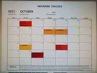
Thank you for responding so quickly. I'm not exactly sure what all this means. I do apologize. I am not as experienced with excel as I'd like to be. I have attached a screenshot of my layout. I tried several times to do the XL2BB but it never worked. It caused my excel to freeze...with dutch names for the month
Roykana.xlsb
A B C D 1 month option1 option2 option3 2 januari - - - 3 februari - - - 4 maart 9 9 12 5 april - - - 6 mei - - - 7 juni - - - 8 juli - - - 9 augustus - - - 10 september - - - 11 oktober - - - 12 november - - - 13 december - - - 14 december - - -
Cell Formulas Range Formula A2:A14 A2 =TEXT((ROW()-1)*28,"mmmm") B2:D14 B2 =IFERROR(COUNTIF(INDIRECT("'"&$A2&"'!$B$2:$B$32"),B$1),"-")
month March (dutch : maart)
Roykana.xlsb
A B 1 day option 2 1 option1 3 2 option3 4 3 option3 5 4 option2 6 5 option2 7 6 option1 8 7 option3 9 8 option3 10 9 option3 11 10 option3 12 11 option3 13 12 option2 14 13 option3 15 14 option1 16 15 option1 17 16 option2 18 17 option1 19 18 option3 20 19 option3 21 20 option2 22 21 option2 23 22 option1 24 23 option1 25 24 option2 26 25 option1 27 26 option3 28 27 option3 29 28 option1 30 29 option2 31 30 option2
Attachments
Upvote
0
with dutch names for the month
Roykana.xlsb
A B C D 1 month option1 option2 option3 2 januari - - - 3 februari - - - 4 maart 9 9 12 5 april - - - 6 mei - - - 7 juni - - - 8 juli - - - 9 augustus - - - 10 september - - - 11 oktober - - - 12 november - - - 13 december - - - 14 december - - -
Cell Formulas Range Formula A2:A14 A2 =TEXT((ROW()-1)*28,"mmmm") B2:D14 B2 =IFERROR(COUNTIF(INDIRECT("'"&$A2&"'!$B$2:$B$32"),B$1),"-")
month March (dutch : maart)
Roykana.xlsb
A B 1 day option 2 1 option1 3 2 option3 4 3 option3 5 4 option2 6 5 option2 7 6 option1 8 7 option3 9 8 option3 10 9 option3 11 10 option3 12 11 option3 13 12 option2 14 13 option3 15 14 option1 16 15 option1 17 16 option2 18 17 option1 19 18 option3 20 19 option3 21 20 option2 22 21 option2 23 22 option1 24 23 option1 25 24 option2 26 25 option1 27 26 option3 28 27 option3 29 28 option1 30 29 option2 31 30 option2
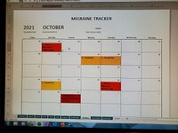
This is a better photo showing the grids. Thanks again for your assistance!with dutch names for the month
Roykana.xlsb
A B C D 1 month option1 option2 option3 2 januari - - - 3 februari - - - 4 maart 9 9 12 5 april - - - 6 mei - - - 7 juni - - - 8 juli - - - 9 augustus - - - 10 september - - - 11 oktober - - - 12 november - - - 13 december - - - 14 december - - -
Cell Formulas Range Formula A2:A14 A2 =TEXT((ROW()-1)*28,"mmmm") B2:D14 B2 =IFERROR(COUNTIF(INDIRECT("'"&$A2&"'!$B$2:$B$32"),B$1),"-")
month March (dutch : maart)
Roykana.xlsb
A B 1 day option 2 1 option1 3 2 option3 4 3 option3 5 4 option2 6 5 option2 7 6 option1 8 7 option3 9 8 option3 10 9 option3 11 10 option3 12 11 option3 13 12 option2 14 13 option3 15 14 option1 16 15 option1 17 16 option2 18 17 option1 19 18 option3 20 19 option3 21 20 option2 22 21 option2 23 22 option1 24 23 option1 25 24 option2 26 25 option1 27 26 option3 28 27 option3 29 28 option1 30 29 option2 31 30 option2
Attachments
Upvote
0
BSALV
Banned user
- Joined
- Oct 31, 2010
- Messages
- 1,651
- Office Version
- 365
- 2013
- 2007
photos weren't very good to see what's in the cells.
So, a month is 5-6 rows of 7 cells and in every cell, there are several things written. Is that more text then those 3 options ?
By the way, select a range, click on xl2bb and click on the ribbon "mini sheet".
Wait a moment for the messagebox "mini sheet succesfully saved in the clipboard", return to Mr Excel and paste (CTRL-V) the clipboard in your answer (it seems like a lot of mystery-code) but after "post reply", it looks oké.
Upvote
0
photos weren't very good to see what's in the cells.
So, a month is 5-6 rows of 7 cells and in every cell, there are several things written. Is that more text then those 3 options ?
By the way, select a range, click on xl2bb and click on the ribbon "mini sheet".
Wait a moment for the messagebox "mini sheet succesfully saved in the clipboard", return to Mr Excel and paste (CTRL-V) the clipboard in your answer (it seems like a lot of mystery-code) but after "post reply", it looks oké.
| Vet Migraine Tracker v2.0.xlsx | |||
|---|---|---|---|
| C | |||
| 8 | 3= Severe Migraine: Debilitating. Unable To Function. | ||
October | |||
| Cells with Conditional Formatting | ||||
|---|---|---|---|---|
| Cell | Condition | Cell Format | Stop If True | |
| B8:H8,B10:H10,B12:H12,B14:H14,B16:H16,B18:H18 | Cell Value | contains "Severe" | text | NO |
| B8:H8,B10:H10,B12:H12,B14:H14,B16:H16,B18:H18 | Cell Value | contains "Moderate" | text | NO |
| B8:H8,B10:H10,B12:H12,B14:H14,B16:H16,B18:H18 | Cell Value | contains "Headache" | text | NO |
Upvote
0
I'll be adding the graph to a new worksheet named graphic representation of attacks. Let me know if you need anything further. Thank you again!
Vet Migraine Tracker v2.0.xlsx
C 8 3= Severe Migraine: Debilitating. Unable To Function.
Cells with Conditional Formatting Cell Condition Cell Format Stop If True B8:H8,B10:H10,B12:H12,B14:H14,B16:H16,B18:H18 Cell Value contains "Severe" text NO B8:H8,B10:H10,B12:H12,B14:H14,B16:H16,B18:H18 Cell Value contains "Moderate" text NO B8:H8,B10:H10,B12:H12,B14:H14,B16:H16,B18:H18 Cell Value contains "Headache" text NO
Upvote
0
In each calendar block, there is a dropdown box with three selections. the first is 1= Headache,I'll be adding the graph to a new worksheet named graphic representation of attacks. Let me know if you need anything further. Thank you again!
2= Moderate Migraine, 3= Severe Migraine
Upvote
0
BSALV
Banned user
- Joined
- Oct 31, 2010
- Messages
- 1,651
- Office Version
- 365
- 2013
- 2007
i don't find it for the moment, to count only the even rows, so i hope here are no texts with sever, moderate or headache in the uneven rows.
the names of the months should be in your local language, not in dutch because of the formula used.
| Roykana.xlsb | ||||||
|---|---|---|---|---|---|---|
| A | B | C | D | |||
| 1 | month | severe | moderate | headache | ||
| 2 | januari | - | - | - | ||
| 3 | februari | - | - | - | ||
| 4 | maart | 1 | 2 | 1 | ||
| 5 | april | - | - | - | ||
| 6 | mei | - | - | - | ||
| 7 | juni | - | - | - | ||
| 8 | juli | - | - | - | ||
| 9 | augustus | - | - | - | ||
| 10 | september | - | - | - | ||
| 11 | oktober | - | - | - | ||
| 12 | november | - | - | - | ||
| 13 | december | - | - | - | ||
| 14 | december | - | - | - | ||
total | ||||||
| Cell Formulas | ||
|---|---|---|
| Range | Formula | |
| A2:A14 | A2 | =TEXT((ROW()-1)*28,"mmmm") |
| B2:D14 | B2 | =IFERROR(COUNTIF(INDIRECT("'"&$A2&"'!$B$8:$H$18"),"*" & B$1& "*"),"-") |
Upvote
0
Solution
Similar threads
- Question
- Replies
- 0
- Views
- 389
- Question
- Replies
- 0
- Views
- 215
- Question
- Replies
- 1
- Views
- 160


