Group number of purchased SKUs by counting customer

blader1989 · Mar 25, 2024

Hi all,

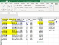
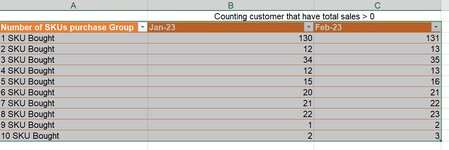
I'm building a report that will group the number of purchased SKUs by counting customer with total sales > 0, I have tried pivot and many ways but I could not get the result as my expectation in attached file so I hope you can help me.

Thank you for your reading time, your help will be most appreciated!!!

Here is my table example

Product Name	Customer Code	Billing Date	Qty	Year	Month	Total Sales
Product 45	121001076	08/02/2023	5	2023	2	864285
Product 46	121001076	04/01/2023	10	2023	1	2033330
Product 46	121001076	01/02/2023	20	2023	2	4066660
Product 51	121001258	20/02/2023	60	2023	2	3914280
Product 51	121001258	24/02/2023	30	2023	2	1957140
Product 51	121001792	04/01/2023	131	2023	1	8546178
Product 51	121001792	09/01/2023	69	2023	1	4501422
Product 51	121001943	04/01/2023	-50	2023	1	-3261900
Product 51	121001943	23/02/2023	50	2023	2	3261900
Product 44	121002462	14/01/2023	10	2023	1	1000000
Product 44	121002462	28/02/2023	20	2023	2	2000000
Product 46	121002462	14/01/2023	10	2023	1	2033330
Product 46	121002462	28/02/2023	20	2023	2	4066660
Product 46	121002507	14/01/2023	20	2023	1	4066660
Product 51	121002507	16/02/2023	20	2023	2	1304760
Product 46	121002535	07/02/2023	4	2023	2	813332
Product 19	121002730	13/02/2023	10	2023	2	985710
Product 44	121002730	10/01/2023	20	2023	1	2000000
Product 44	121002730	27/01/2023	30	2023	1	3000000
Product 44	121002730	13/02/2023	30	2023	2	3000000
Product 44	121002730	23/02/2023	30	2023	2	3000000
Product 44	121002730	28/02/2023	20	2023	2	2000000
Product 46	121002730	10/01/2023	20	2023	1	4066660
Product 46	121002730	27/01/2023	30	2023	1	6099990
Product 46	121002730	31/01/2023	10	2023	1	2033330
Product 46	121002730	31/01/2023	10	2023	1	2033330
Product 46	121002730	13/02/2023	20	2023	2	4066660
Product 46	121002730	23/02/2023	20	2023	2	4066660
Product 46	121002730	28/02/2023	10	2023	2	2033330
Product 46	121002752	14/01/2023	10	2023	1	2033330
Product 44	121003038	05/01/2023	20	2023	1	2000000
Product 44	121003038	21/02/2023	20	2023	2	2000000
Product 44	121003038	24/02/2023	20	2023	2	2000000
Product 46	121003038	05/01/2023	25	2023	1	5083325
Product 46	121003038	27/01/2023	20	2023	1	4066660
Product 46	121003038	28/01/2023	10	2023	1	2033330
Product 46	121003038	21/02/2023	10	2023	2	2033330
Product 46	121003038	24/02/2023	20	2023	2	4066660
Product 44	121003326	16/01/2023	10	2023	1	1000000
Product 44	121003326	27/01/2023	30	2023	1	3000000
Product 51	121003349	17/02/2023	50	2023	2	3261900
Product 51	121003359	16/01/2023	41	2023	1	2674758
Product 44	121003423	16/01/2023	10	2023	1	1000000
Product 44	121003423	27/01/2023	20	2023	1	2000000
Product 46	121003423	16/01/2023	30	2023	1	6099990
Product 46	121003423	27/01/2023	30	2023	1	6099990
Product 44	121003739	09/01/2023	5	2023	1	500000
Product 44	121003739	15/02/2023	5	2023	2	500000
Product 46	121003739	09/01/2023	5	2023	1	1016665

dermie_72 · Mar 25, 2024

Not sure if this is what you're after:
I put your sample data into a spreadsheet A1:G50
I created a unique table of Customer codes via the unique function into I2

Excel Formula:

=UNIQUE(B2:B50)

Then copied the month's from the table to the heading, IE J1:K1 became 1 & 2
I then used a formula to count the number of sku's purchased by customer that month.

Excel Formula:

=COUNTIFS($B:$B,$I2,$F:$F,J$1,$D:$D,">0")

And encompassed the range you're wanting to detect.
In Q2 I added the Number of SKU's going from 1 down and used a formula in R2 going across the number of months (You might need to change the start column depending on the number of months in the previous table.

Excel Formula:

=COUNTIF(J$:J$,$Q2)

This returns the table that you requested. Hope that helps.

blader1989 · Mar 26, 2024

dermie_72 said:
Not sure if this is what you're after:
I put your sample data into a spreadsheet A1:G50
I created a unique table of Customer codes via the unique function into I2

Excel Formula:

=UNIQUE(B2:B50)

Then copied the month's from the table to the heading, IE J1:K1 became 1 & 2
I then used a formula to count the number of sku's purchased by customer that month.

Excel Formula:

=COUNTIFS($B:$B,$I2,$F:$F,J$1,$D:$D,">0")

And encompassed the range you're wanting to detect.
In Q2 I added the Number of SKU's going from 1 down and used a formula in R2 going across the number of months (You might need to change the start column depending on the number of months in the previous table.

Excel Formula:

=COUNTIF(J$:J$,$Q2)

This returns the table that you requested. Hope that helps.

Hi Dermie,

Thank you so much, that's look promising, I have applied your approach and found how can I modify that if they buy same product, it will only count as 1? In the image below you can see this customer code 121002730 buy only 2 product even he/she bought in multiple times.

Peter_SSs · Mar 26, 2024

@blader1989
It would help you get better/faster replies if you could give your sample data in a form helpers can easily test with.

I suggest that you investigate XL2BB for providing sample data to make it easier for helpers by not having to manually type out sample data to test with.

Try a formula like this in J2 for the layout shown in post #3

Excel Formula:

=BYROW(I2:I4,LAMBDA(r,IFNA(ROWS(UNIQUE(FILTER(A2:A50,B2:B50=r,NA()))),0)))

blader1989 · Mar 26, 2024

Peter_SSs said:
@blader1989
It would help you get better/faster replies if you could give your sample data in a form helpers can easily test with.
I suggest that you investigate XL2BB for providing sample data to make it easier for helpers by not having to manually type out sample data to test with.

Try a formula like this in J2 for the layout shown in post #3

Excel Formula:

=BYROW(I2:I4,LAMBDA(r,IFNA(ROWS(UNIQUE(FILTER(A2:A50,B2:B50=r,NA()))),0)))

Hi Peter,

Thank you so much. I have tried your code by it didn't show anything so I copy with XL2BB for you to check

Book1.xlsx

A

B

C

D

E

F

G

H

I

J

1

Product Name

Customer Code

Billing Date

Qty

Year

Month

Total Sales

Jan

2

Product 44

121002462

14/01/2023

10

2023

1

1000000

121002462

2

3

Product 44

121002730

10/01/2023

20

2023

1

2000000

121002730

#SPILL!

4

Product 44

121002730

27/01/2023

30

2023

1

3000000

121003038

1

5

Product 44

121003038

05/01/2023

20

2023

1

2000000

121001076

1

6

Product 46

121001076

04/01/2023

10

2023

1

2033330

121002507

1

7

Product 46

121002462

14/01/2023

10

2023

1

2033330

121002752

1

8

Product 46

121002507

14/01/2023

20

2023

1

4066660

121001792

2

9

Product 46

121002730

10/01/2023

20

2023

1

4066660

121001943

0

10

Product 46

121002730

27/01/2023

30

2023

1

6099990

11

Product 46

121002730

31/01/2023

10

2023

1

2033330

12

Product 46

121002730

31/01/2023

10

2023

1

2033330

13

Product 46

121002752

14/01/2023

10

2023

1

2033330

14

Product 51

121001792

04/01/2023

131

2023

1

8546178

15

Product 51

121001792

09/01/2023

69

2023

1

4501422

16

Product 51

121001943

04/01/2023

-50

2023

1

-3261900

Sheet2

Cell Formulas
Range	Formula
I2:I9	I2	=UNIQUE(B2:B16)
J2,J4:J9	J2	=COUNTIFS($B:$B,$I2,$G:$G,">0")
J3	J3	=BYROW(I2:I9,LAMBDA(r,IFNA(ROWS(UNIQUE(FILTER(A2:A16,B2:B16=r,NA()))),0)))
Dynamic array formulas.

Peter_SSs · Mar 26, 2024

Thanks for the XL2BB data - makes it much easier.

You put the formula in J3 not J2 as suggested. Put it in J2 instead and remove all the formulas from J3 to J9.

Also, since you have a dynamic array formula in I2, change the J2 formula to this, then you do not have to specify the column I range.

Excel Formula:

=BYROW(I2#,LAMBDA(r,IFNA(ROWS(UNIQUE(FILTER(A2:A16,B2:B16=r,NA()))),0)))

blader1989 · Mar 26, 2024

Hi @dermie_72 and @Peter_SSs

Thank you so much for your help, it nearly solved my problem at 99%, only 1% at how can we include the condition that the total value of purchased product should be large than 0 in post# 2 (=COUNTIFS($B:$B,$I2,$F:$F,J$1,$D:$D,">0"))? Because in our scenario, when customer returned the product, it will show the negative in the report. Like the table below, the customer code 121002730 when counting purchased product should be 1 because the product 44 purchased by he/she was 0 -> means the product was return due to any reason.

Book1_SKU purchased segment.xlsx

A

B

C

D

E

F

G

H

I

J

K

1

Product Name

Customer Code

Billing Date

Qty

Year

Month

Total Sales

Jan

2

Product 44

121002462

14/01/2023

10

2023

1

1000000

121002462

2

3

Product 44

121002730

10/01/2023

20

2023

1

2000000

121002730

2

should be 1

4

Product 44

121002730

11/01/2023

-20

2023

1

-2000000

121003038

1

5

Product 44

121003038

05/01/2023

20

2023

1

2000000

121001076

1

6

Product 46

121001076

04/01/2023

10

2023

1

2033330

121002507

1

7

Product 46

121002462

14/01/2023

10

2023

1

2033330

121002752

1

8

Product 46

121002507

14/01/2023

20

2023

1

4066660

121001792

1

9

Product 46

121002730

10/01/2023

20

2023

1

4066660

121001943

1

10

Product 46

121002730

27/01/2023

30

2023

1

6099990

11

Product 46

121002730

31/01/2023

10

2023

1

2033330

12

Product 46

121002730

31/01/2023

10

2023

1

2033330

13

Product 46

121002752

14/01/2023

10

2023

1

2033330

14

Product 51

121001792

04/01/2023

131

2023

1

8546178

15

Product 51

121001792

09/01/2023

69

2023

1

4501422

16

Product 51

121001943

04/01/2023

-50

2023

1

-3261900

Sheet2

Cell Formulas
Range	Formula
I2:I9	I2	=UNIQUE(B2:B16)
J2:J9	J2	=BYROW(I2#,LAMBDA(r,IFNA(ROWS(UNIQUE(FILTER(A2:A16,B2:B16=r,NA()))),0)))
Dynamic array formulas.

Peter_SSs · Mar 27, 2024

blader1989 said:
the customer code 121002730 when counting purchased product should be 1 because the product 44 purchased by he/she was 0

So the count for customer code 121001943 should also be zero since that code has a negative total sales?

blader1989.xlsm

A

B

G

H

I

J

K

1

Product Name

Customer Code

Total Sales

Jan

2

Product 44

121002462

1000000

121002462

2

3

Product 44

121002730

2000000

121002730

1

should be 1

4

Product 44

121002730

-2000000

121003038

1

5

Product 44

121003038

2000000

121001076

1

6

Product 46

121001076

2033330

121002507

1

7

Product 46

121002462

2033330

121002752

1

8

Product 46

121002507

4066660

121001792

1

9

Product 46

121002730

4066660

121001943

0

??

10

Product 46

121002730

6099990

11

Product 46

121002730

2033330

12

Product 46

121002730

2033330

13

Product 46

121002752

2033330

14

Product 51

121001792

8546178

15

Product 51

121001792

4501422

16

Product 51

121001943

-3261900

17

Sheet2

Cell Formulas
Range	Formula
I2:I9	I2	=UNIQUE(B2:B16)
J2:J9	J2	=BYROW(I2#,LAMBDA(r,IFNA(ROWS(UNIQUE(FILTER(A2:A16,(B2:B16=r)*(SUMIFS(G2:G16,A2:A16,A2:A16,B2:B16,r)>0),NA()))),0)))
Dynamic array formulas.

dermie_72 · Mar 27, 2024

Excel Formula:

=BYROW(I2#,LAMBDA(r,IFNA(ROWS(UNIQUE(FILTER(A2:A16,B2:B16=r,D2:D16=">0",NA()))),0)))

You wanted to only have items with a positive value in D, so you would need to include that in your filter

Peter_SSs · Mar 27, 2024

@dermie_72
That isn't a valid formula.

dermie_72 said:
You wanted to only have items with a positive value in D,

Also, I think the OP does not want just rows with positive value but customers who have positive total for a product in D

Group number of purchased SKUs by counting customer

blader1989

New Member

Attachments

Excel Facts

dermie_72

Well-known Member

blader1989

New Member

Peter_SSs

MrExcel MVP, Moderator

blader1989

New Member

Peter_SSs

MrExcel MVP, Moderator

blader1989

New Member

Attachments

Peter_SSs

MrExcel MVP, Moderator

dermie_72

Well-known Member

Peter_SSs

MrExcel MVP, Moderator

Similar threads

Forum statistics

Share this page

Group number of purchased SKUs by counting customer

New Member

Attachments

Excel Facts

Well-known Member

New Member

MrExcel MVP, Moderator

New Member

MrExcel MVP, Moderator

New Member

Attachments

MrExcel MVP, Moderator

Well-known Member

MrExcel MVP, Moderator

Similar threads

Forum statistics

Share this page

We've detected that you are using an adblocker.

Which adblocker are you using?

Disable AdBlock

Disable AdBlock Plus

Disable uBlock Origin

Disable uBlock