Grouping Data

[KarthickDijo]

Hi All,

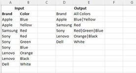
I need to group few data (in a column) based on the another column. Kindly help me out how it can be done apart from VBA. Attached the sample input and output.

Thanks in advance

 

[Jimmypop]

Hi there

Not sure if this will work for you?

Book1
	A	B	C	D	E
1	Input
2	Brand	Color		Brand	All Colours
3	Apple	Blue		Apple	Blue|Yellow
4	Apple	Yellow		Samsung	Red
5	Samsung	Red		Sony	Red|Green|Blue
6	Sony	Red		Lenovo	Orange|Black
7	Sony	Green		Dell	White
8	Sony	Blue
9	Lenovo	Orange
10	Lenovo	Black
11	Dell	White
Sheet1

Cell Formulas
Range	Formula
D3:D7	D3	=FILTER(A3:A12,(B3:B12>=A1),"NA")
E3:E7	E3	=TEXTJOIN("|",TRUE,IF(A3:A11=D3,B3:B11,""))
Dynamic array formulas.

 

[Fluff]

Welcome to the MrExcel Message Board!

Cross-posting (posting the same question in more than one forum) is not against our rules, but the method of doing so is covered by #13 of the Forum Rules.

Be sure to follow & read the link at the end of the rule too!

Cross posted at: Grouping Data
If you have posted the question at more places, please provide links to those as well.

If you do cross-post in the future and also provide links, then there shouldn’t be a problem.

 

[Fluff]

Another option for xl2019

Excel Doubt.xlsx
	A	B	C	D	E
1	Brand	Color		Brand	All Colors
2	Apple	Blue		Apple	Blue|Yellow
3	Apple	Yellow		Samsung	Red
4	Samsung	Red		Sony	Red|Green|Blue
5	Sony	Red		Lenovo	Orange|Black
6	Sony	Green		Dell	White
7	Sony	Blue
8	Lenovo	Orange
9	Lenovo	Black
10	Dell	White
11
Sheet1

Cell Formulas
Range	Formula
D2:D8	D2	=IFERROR(INDEX($A$2:$A$10,AGGREGATE(15,6,(ROW($A$2:$A$10)-ROW($A$2)+1)/(ISNA(MATCH($A$2:$A$10,D$1:D1,0))),1)),"")
E2:E8	E2	=IF(D2="","",TEXTJOIN("|",,IF(A2:A10=D2,B2:B10,"")))

 

[KarthickDijo]

Hi there

Not sure if this will work for you?

Book1
	A	B	C	D	E
1	Input
2	Brand	Color		Brand	All Colours
3	Apple	Blue		Apple	Blue|Yellow
4	Apple	Yellow		Samsung	Red
5	Samsung	Red		Sony	Red|Green|Blue
6	Sony	Red		Lenovo	Orange|Black
7	Sony	Green		Dell	White
8	Sony	Blue
9	Lenovo	Orange
10	Lenovo	Black
11	Dell	White
Sheet1

Cell Formulas
Range	Formula
D3:D7	D3	=FILTER(A3:A12,(B3:B12>=A1),"NA")
E3:E7	E3	=TEXTJOIN("|",TRUE,IF(A3:A11=D3,B3:B11,""))
Dynamic array formulas.

Thanks a lot for the help !!

 

[KarthickDijo]

Another option for xl2019

Excel Doubt.xlsx
	A	B	C	D	E
1	Brand	Color		Brand	All Colors
2	Apple	Blue		Apple	Blue|Yellow
3	Apple	Yellow		Samsung	Red
4	Samsung	Red		Sony	Red|Green|Blue
5	Sony	Red		Lenovo	Orange|Black
6	Sony	Green		Dell	White
7	Sony	Blue
8	Lenovo	Orange
9	Lenovo	Black
10	Dell	White
11
Sheet1

Cell Formulas
Range	Formula
D2:D8	D2	=IFERROR(INDEX($A$2:$A$10,AGGREGATE(15,6,(ROW($A$2:$A$10)-ROW($A$2)+1)/(ISNA(MATCH($A$2:$A$10,D$1:D1,0))),1)),"")
E2:E8	E2	=IF(D2="","",TEXTJOIN("|",,IF(A2:A10=D2,B2:B10,"")))

Thanks for the help !! Just one clarification, why can't we use "UNIQUE" function in the D2 cell.

 

[RoryA]

2019 doesn't have UNIQUE as far as I am aware.

You could also use Power Pivot to produce the result table.

 

[KarthickDijo]

2019 doesn't have UNIQUE as far as I am aware.

You could also use Power Pivot to produce the result table.

Thanks for the info. Am not aware of power pivot, however will try to learn that asap. If possible kindly explain me how it can be done.

 

[RoryA]

Turn the data into a table and load it into the data model using the Power Pivot tab. Then create a power pivot table and add a measure like:

=CONCATENATEX(VALUES(Table1[Color]),[Color],"|")

where Table1 is the name of the table you created at the start.

 

[Jimmypop]

Another option for xl2019

Excel Doubt.xlsx
	A	B	C	D	E
1	Brand	Color		Brand	All Colors
2	Apple	Blue		Apple	Blue|Yellow
3	Apple	Yellow		Samsung	Red
4	Samsung	Red		Sony	Red|Green|Blue
5	Sony	Red		Lenovo	Orange|Black
6	Sony	Green		Dell	White
7	Sony	Blue
8	Lenovo	Orange
9	Lenovo	Black
10	Dell	White
11
Sheet1

Cell Formulas
Range	Formula
D2:D8	D2	=IFERROR(INDEX($A$2:$A$10,AGGREGATE(15,6,(ROW($A$2:$A$10)-ROW($A$2)+1)/(ISNA(MATCH($A$2:$A$10,D$1:D1,0))),1)),"")
E2:E8	E2	=IF(D2="","",TEXTJOIN("|",,IF(A2:A10=D2,B2:B10,"")))

Hi Fluff... and apologies to OP for sort of hijacking this thread but I have a quick question... when working out the formula earlier... why does the below give me two options for "Sony" and not a unique list of values...

Book3.xlsx
	A	B	C	D	E
1	Input
2	Brand	Color		Brand	All Colours
3	Apple	Blue		Apple	Blue | Yellow
4	Apple	Yellow		Samsung	Red
5	Samsung	Red		Sony	Red|Green|Blue
6	Sony	Red		Sony	Red|Green|Blue
7	Sony	Green		Lenovo	Orange|Black
8	Sony	Blue		Dell
9	Lenovo	Orange
10	Lenovo	Black
11	Dell	White
Sheet1

Cell Formulas
Range	Formula
D3:D8	D3	=FILTER(A3:A11,(B3:B11>=A2),"NA")
E3	E3	=TEXTJOIN(" | ",TRUE,IF(A3:A11=D3,B3:B11,""))
E4:E7	E4	=TEXTJOIN("|",TRUE,IF(A4:A12=D4,B4:B12,""))
Dynamic array formulas.