Having issues with Formula!!!

JB2385

New Member
Joined
Apr 26, 2023
Messages
11
Office Version
  1. 365
Platform
  1. Windows
I am going to break down how I am understanding a portion of this formula below thus will lead to my question.

Formula:

=IF(AND(B$13<>"",$A14<>""),SUMPRODUCT((SUBSTITUTE($A$3:$A$10,"1/","")=TRIM(SUBSTITUTE($A14,"Site","")))*($D$3:$D$10=B$13)),"")

The portions of the formula =TRIM(SUBSTITUTE($A14,"Site","") is essential taking out "Site" from the cell and leaving the Site number and in this case its reading it as 1 instead of Site 1. Please correct me if I am wrong.

My question is how can I had a second =Trim(substitute like above or do I not need it? My assumption would be like this (below). Again correct me if I am wrong.

=IF(AND(F$13<>"",$A14<>""),SUMPRODUCT((SUBSTITUTE($A$3:$A$10,"/5","")=TRIM(SUBSTITUTE($A14,"Site","")=TRIM(SUBSTITUTE($F13,"Ford 1.1","")))*($E$3:$E$10=F$13)),""))

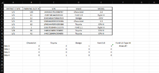
In my master tracker I have another substitution I need input in F14 and the example above is how I was thinking it would be implemented however, I am receiving #VALUE! in the cell F14 instead of the number. The "Ford 1.1" is what I am trying to substitute so the formula will only count Type III instead of "Ford 1.1". I am using the first formula in all my other cells except column F. I hope this was descriptive enough. Please let me know if there any questions.
 

Attachments

  • formula 3.png
    formula 3.png
    31.2 KB · Views: 8

Excel Facts

Highlight Duplicates
Home, Conditional Formatting, Highlight Cells, Duplicate records, OK to add pink formatting to any duplicates in selected range.
Maybe
Excel Formula:
=IF(AND(F$13<>"",$A14<>""),SUMPRODUCT((SUBSTITUTE($A$3:$A$10,"/5","")=TRIM(SUBSTITUTE($A14,"Site",""))*($E$3:$E$10=TRIM(SUBSTITUTE($F13,"Ford 1.1","")))),""))
 
Upvote 0
Maybe
Excel Formula:
=IF(AND(F$13<>"",$A14<>""),SUMPRODUCT((SUBSTITUTE($A$3:$A$10,"/5","")=TRIM(SUBSTITUTE($A14,"Site",""))*($E$3:$E$10=TRIM(SUBSTITUTE($F13,"Ford 1.1","")))),""))
Thank you for the quick reply. It gave me the same #Value! error.
 
Upvote 0
In that case can you post your data.

MrExcel has a tool called “XL2BB” that lets you post samples of your data that will allow us to copy/paste it to our Excel spreadsheets, so we can work with the same copy of data that you are. Instructions on using this tool can be found here: XL2BB Add-in

Note that there is also a "Test Here” forum on this board. This is a place where you can test using this tool (or any other posting techniques that you want to test) before trying to use those tools in your actual posts.


This is what I am working with.


Vehicle Inventory 4.xlsx
ABCDEF
1
2DISTRICT / SITEPARKING SLOT #VINMAKEMODEL
31/1120JH4KA3170LC006787Chevrolet2.6
41/111JS1RF16C442100152Ford 1.1Type III
51/1122C4GM68475R667819DodgeORV
61/1651P4GH44R0RX359386Chevrolet2.1
71/1121P4GH44R0RX359386ToyotaORV II
81/111GBJ7D1B4BV132373Ford 1.0Type III
91/466JH4KA2640GC004861ToyotaORV II
101/141JH4CC2640NC004693ToyotaORV II
11
12
13ChevroletToyotaDodgeFord 1.0Ford 1.1 Type III
14Site 12211#VALUE!
15Site 20000
16Site 30000
17Site 40100
Sheet1
Cell Formulas
RangeFormula
B14:E17B14=IF(AND(B$13<>"",$A14<>""),SUMPRODUCT((SUBSTITUTE($A$3:$A$10,"1/","")=TRIM(SUBSTITUTE($A14,"Site","")))*($D$3:$D$10=B$13)),"")
F14F14=IF(AND(F$13<>"",$A14<>""),SUMPRODUCT((SUBSTITUTE($A$3:$A$10,"/5","")=TRIM(SUBSTITUTE($A14,"Site",""))*($E$3:$E$10=TRIM(SUBSTITUTE($F13,"Ford 1.1","")))),""))
 
Upvote 0
Thanks for that, how about
Fluff.xlsm
ABCDEF
1
2DISTRICT / SITEPARKING SLOT #VINMAKEMODEL
31/1120JH4KA3170LC006787Chevrolet2.6
41/111JS1RF16C442100152Ford 1.1Type III
51/1122C4GM68475R667819DodgeORV
61/1651P4GH44R0RX359386Chevrolet2.1
71/1121P4GH44R0RX359386ToyotaORV II
81/111GBJ7D1B4BV132373Ford 1.0Type III
91/466JH4KA2640GC004861ToyotaORV II
101/141JH4CC2640NC004693ToyotaORV II
11
12
13ChevroletToyotaDodgeFord 1.0Ford 1.1 Type III
14Site 122112
15Site 200000
16Site 300000
17Site 401000
Dashboard
Cell Formulas
RangeFormula
B14:E17B14=IF(AND(B$13<>"",$A14<>""),SUMPRODUCT((SUBSTITUTE($A$3:$A$10,"1/","")=TRIM(SUBSTITUTE($A14,"Site","")))*($D$3:$D$10=B$13)),"")
F14F14=IF(AND(F$13<>"",$A14<>""),SUMPRODUCT((SUBSTITUTE($A$3:$A$10,"1/","")=TRIM(SUBSTITUTE($A14,"Site","")))*($E$3:$E$10=TRIM(SUBSTITUTE($F13,"Ford 1.1","")))),"")
F15:F17F15=IF(AND(F$13<>"",$A15<>""),SUMPRODUCT((SUBSTITUTE($A$3:$A$10,"/5","")=TRIM(SUBSTITUTE($A15,"Site","")))*($E$3:$E$10=TRIM(SUBSTITUTE($F14,"Ford 1.1","")))),"")
Thank you for the quick response. It looks like its picking up 2 Ford 1.1 Type III for Site 1. There is only 1. I think it is picking up the Ford 1.0 Type III and the Ford 1.1 Type III.
 
Upvote 0
In that case try
Excel Formula:
=IF(AND(F$13<>"",$A14<>""),SUMPRODUCT((SUBSTITUTE($A$3:$A$10,"1/","")=TRIM(SUBSTITUTE($A14,"Site","")))*($D$3:$D$10="ford 1.1")*($E$3:$E$10=TRIM(SUBSTITUTE($F13,"Ford 1.1","")))),"")
 
Upvote 1
Solution
Thank you for the quick response. It looks like its picking up 2 Ford 1.1 Type III for Site 1. There is only 1. I think it is picking up the Ford 1.0 Type III and the Ford 1.1 Type III.

In that case try
Excel Formula:
=IF(AND(F$13<>"",$A14<>""),SUMPRODUCT((SUBSTITUTE($A$3:$A$10,"1/","")=TRIM(SUBSTITUTE($A14,"Site","")))*($D$3:$D$10="ford 1.1")*($E$3:$E$10=TRIM(SUBSTITUTE($F13,"Ford 1.1","")))),"")
Word perfectly!!!! Thank you so much! Issue resolved.
 
Upvote 0
You're welcome & thanks for the feedback.
 
Upvote 0

Forum statistics

Threads
1,215,475
Messages
6,125,028
Members
449,205
Latest member
Eggy66

We've detected that you are using an adblocker.

We have a great community of people providing Excel help here, but the hosting costs are enormous. You can help keep this site running by allowing ads on MrExcel.com.
Allow Ads at MrExcel

Which adblocker are you using?

Disable AdBlock

Follow these easy steps to disable AdBlock

1)Click on the icon in the browser’s toolbar.
2)Click on the icon in the browser’s toolbar.
2)Click on the "Pause on this site" option.
Go back

Disable AdBlock Plus

Follow these easy steps to disable AdBlock Plus

1)Click on the icon in the browser’s toolbar.
2)Click on the toggle to disable it for "mrexcel.com".
Go back

Disable uBlock Origin

Follow these easy steps to disable uBlock Origin

1)Click on the icon in the browser’s toolbar.
2)Click on the "Power" button.
3)Click on the "Refresh" button.
Go back

Disable uBlock

Follow these easy steps to disable uBlock

1)Click on the icon in the browser’s toolbar.
2)Click on the "Power" button.
3)Click on the "Refresh" button.
Go back
Back
Top