Having trouble getting a date

jthomas3029

New Member
Joined
Jun 29, 2020
Messages
30
Office Version
  1. 2010
Platform
  1. Windows
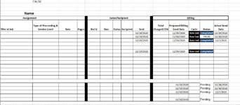
I have a proposed billing date (A1) and a status (B1) and (C1) actual send date. My formula for B1 is: =IF(AND(A1>=TODAY(),"Pending"),IF(AND(C1<>A1),"completed")). To be sure it is "volatile". The concept is to alert the user to the upcoming send date, A1, hence "pending", but once it is sent ,C1, to change the pending to "completed" in B1 I had a vlookup that worked for me based on a countdown model to TODAY which then reported completed but the user wants "completed" when the send date meets or exceeds the proposed billing date. Each of the formulas work well independently, it is when they are combined there a volatile explosion.
 

Excel Facts

Can you AutoAverage in Excel?
There is a drop-down next to the AutoSum symbol. Open the drop-down to choose AVERAGE, COUNT, MAX, or MIN
Why are you using AND() for single criteria, is there more to the formula that you have not shown?

It looks like you have some misplaced parentheses, possibly resulting from the superfluous AND() functions, correcting those may help.
Excel Formula:
=IF(A1>=TODAY(),"Pending",IF(C1<>A1,"completed"))
it may also be necessary to change the logic if it is going to be necessary for "completed" to be shown in some cases where A1 is >=TODAY().
 
Upvote 0
The revised formula also is volatile. I changed the date in C! to see if it made any difference and it does not.
 
Upvote 0
To me, it looks correct based on the information that you have provided. If it is not what is needed then a sample of A1 and C1 combinations with the expected results will be needed for clarification.

Please use XL2BB (see link in my my signature block below) for posting samples, not screen captures.
 
Upvote 0
Not sure what happened there, you need to select all of the cells that you want to post, not just the first one.
 
Upvote 0
Scoping 2020 11 22.xlsm
ABCDEFGHIJKLMNOPQ
1FALSE
2
3
4Name
5AssignmentDates/RecipientBilling
6Title of JobType of Proceeding & Service LevelRatePagesRec'dDueStatusRecipientSentTotal Charged CDNProposed Billing Send DateCycleStatusActual Send Date
7  11/18/202011/30/2020Nov Endcompleted11/24/2020
8  11/19/2020 11/30/2020Nov EndFALSE11/30/2020
9  11/20/2020 11/30/2020Nov Endcompleted12/3/2020
10     
11     
12  11/19/2020 11/30/2020Nov Endcompleted
13  
14  
15     
16      
17      
18      
19      
20
2111/30/2020Pending11/24/2020
2211/30/2020Pending11/30/2020
2311/30/2020Pending12/3/2020
24
2511/30/2020Pending
26
Unassigned (4)
Cell Formulas
RangeFormula
B1B1=IF(A1>=TODAY(),"Pending",IF(C1<>A1,"completed"))
M7M7=IF(J7="","",INDEX(Tables!$K$6:$K$31,SUMPRODUCT(($J$7>=Tables!$L$6:$L$31)*($J$7<=Tables!$M$6:$M$31)*MATCH(ROW(Tables!$K$6:$K$31),ROW(Tables!$K$6:$K$31)))))
N7N7=IF(M7="","",INDEX(Tables!$J$6:$J$32,SUMPRODUCT(($M$7>=Tables!$L$6:$L$32)*($M$7<=Tables!$M$6:$M$32)*MATCH(ROW(Tables!$K$6:$K$32),ROW(Tables!$K$6:$K$32)))))
O12,O7:O9O7=IF(M7<=TODAY(),"Pending",IF(P7<>M7,"completed"))
L15:L19,L8:L12L8=IF((ISERROR(C8*D8))," ",(C8*D8))
M8M8=IF(J8="","",INDEX(Tables!$K$6:$K$30,SUMPRODUCT(($J$8>=Tables!$L$6:$L$30)*($J$8<=Tables!$M$6:$M$30)*MATCH(ROW(Tables!$K$6:$K$30),ROW(Tables!$K$6:$K$30)))))
N8N8=IF(M8="","",INDEX(Tables!$J$6:$J$32,SUMPRODUCT(($M$8>=Tables!$L$6:$L$32)*($M$8<=Tables!$M$6:$M$32)*MATCH(ROW(Tables!$K$6:$K$32),ROW(Tables!$K$6:$K$32)))))
M9M9=IF(J9="","",INDEX(Tables!$K$6:$K$30,SUMPRODUCT(($J$9>=Tables!$L$6:$L$30)*($J$9<=Tables!$M$6:$M$30)*MATCH(ROW(Tables!$K$6:$K$30),ROW(Tables!$K$6:$K$30)))))
N9N9=IF(M9="","",INDEX(Tables!$J$6:$J$32,SUMPRODUCT(($M$9>=Tables!$L$6:$L$32)*($M$9<=Tables!$M$6:$M$32)*MATCH(ROW(Tables!$K$6:$K$32),ROW(Tables!$K$6:$K$32)))))
M10M10=IF(J10="","",INDEX(Tables!$K$6:$K$30,SUMPRODUCT(($J$10>=Tables!$L$6:$L$30)*($J$10<=Tables!$M$6:$M$30)*MATCH(ROW(Tables!$K$6:$K$30),ROW(Tables!$K$6:$K$30)))))
N10N10=IF(M10="","",INDEX(Tables!$J$6:$J$32,SUMPRODUCT(($M$10>=Tables!$L$6:$L$32)*($M$10<=Tables!$M$6:$M$32)*MATCH(ROW(Tables!$K$6:$K$32),ROW(Tables!$K$6:$K$32)))))
M11M11=IF(J11="","",INDEX(Tables!$K$6:$K$30,SUMPRODUCT(($J$11>=Tables!$L$6:$L$30)*($J$11<=Tables!$M$6:$M$30)*MATCH(ROW(Tables!$K$6:$K$30),ROW(Tables!$K$6:$K$30)))))
N11N11=IF(M11="","",INDEX(Tables!$J$6:$J$32,SUMPRODUCT(($M$11>=Tables!$L$6:$L$32)*($M$11<=Tables!$M$6:$M$32)*MATCH(ROW(Tables!$K$6:$K$32),ROW(Tables!$K$6:$K$32)))))
M12M12=IF(J12="","",INDEX(Tables!$K$6:$K$30,SUMPRODUCT(($J$12>=Tables!$L$6:$L$30)*($J$12<=Tables!$M$6:$M$30)*MATCH(ROW(Tables!$K$6:$K$30),ROW(Tables!$K$6:$K$30)))))
N12N12=IF(M12="","",INDEX(Tables!$J$6:$J$32,SUMPRODUCT(($M$12>=Tables!$L$6:$L$32)*($M$12<=Tables!$M$6:$M$32)*MATCH(ROW(Tables!$K$6:$K$32),ROW(Tables!$K$6:$K$32)))))
M15M15=IF(J15="","",INDEX(Tables!$K$6:$K$30,SUMPRODUCT(($J$15>=Tables!$L$6:$L$30)*($J$15<=Tables!$M$6:$M$30)*MATCH(ROW(Tables!$K$6:$K$30),ROW(Tables!$K$6:$K$30)))))
N15N15=IF(M15="","",INDEX(Tables!$J$6:$J$32,SUMPRODUCT(($M$15>=Tables!$L$6:$L$32)*($M$15<=Tables!$M$6:$M$32)*MATCH(ROW(Tables!$K$6:$K$32),ROW(Tables!$K$6:$K$32)))))
M16M16=IF(J16="","",INDEX(Tables!$K$6:$K$30,SUMPRODUCT(($J$16>=Tables!$L$6:$L$30)*($J$16<=Tables!$M$6:$M$30)*MATCH(ROW(Tables!$K$6:$K$30),ROW(Tables!$K$6:$K$30)))))
N16N16=IF(M16="","",INDEX(Tables!$J$6:$J$32,SUMPRODUCT(($M$16>=Tables!$L$6:$L$32)*($M$16<=Tables!$M$6:$M$32)*MATCH(ROW(Tables!$K$6:$K$32),ROW(Tables!$K$6:$K$32)))))
O16:O19O16=IF(M16="","",VLOOKUP(TODAY()-M16,Tables!$E$3:$F$17,2,1))
M17M17=IF(J17="","",INDEX(Tables!$K$6:$K$30,SUMPRODUCT(($J$17>=Tables!$L$6:$L$30)*($J$17<=Tables!$M$6:$M$30)*MATCH(ROW(Tables!$K$6:$K$30),ROW(Tables!$K$6:$K$30)))))
N17N17=IF(M17="","",INDEX(Tables!$J$6:$J$32,SUMPRODUCT(($M$17>=Tables!$L$6:$L$32)*($M$17<=Tables!$M$6:$M$32)*MATCH(ROW(Tables!$K$6:$K$32),ROW(Tables!$K$6:$K$32)))))
M18M18=IF(J18="","",INDEX(Tables!$K$6:$K$30,SUMPRODUCT(($J$18>=Tables!$L$6:$L$30)*($J$18<=Tables!$M$6:$M$30)*MATCH(ROW(Tables!$K$6:$K$30),ROW(Tables!$K$6:$K$30)))))
N18N18=IF(M18="","",INDEX(Tables!$J$6:$J$32,SUMPRODUCT(($M$18>=Tables!$L$6:$L$32)*($M$18<=Tables!$M$6:$M$32)*MATCH(ROW(Tables!$K$6:$K$32),ROW(Tables!$K$6:$K$32)))))
M19M19=IF(J19="","",INDEX(Tables!$K$6:$K$30,SUMPRODUCT(($J$19>=Tables!$L$6:$L$30)*($J$19<=Tables!$M$6:$M$30)*MATCH(ROW(Tables!$K$6:$K$30),ROW(Tables!$K$6:$K$30)))))
N19N19=IF(M19="","",INDEX(Tables!$J$6:$J$32,SUMPRODUCT(($M$19>=Tables!$L$6:$L$32)*($M$19<=Tables!$M$6:$M$32)*MATCH(ROW(Tables!$K$6:$K$32),ROW(Tables!$K$6:$K$32)))))
C7:C19C7=IF(B7="","",VLOOKUP(B7,Tables!$A$3:$B$8,2,FALSE))
H7:H19H7=IF(G7="","",VLOOKUP(TODAY()-G7,Tables!$A$12:$C$26,3,1))
O25,O21:O23O21=IF(M21>=TODAY(),"Pending",IF(P21<>M21,"completed"))
Named Ranges
NameRefers ToCells
'Unassigned (4)'!Billing=Date_Scheduler3436N15:N19, N7:N12
Billing=Date_Scheduler3436N15:N19, N7:N12
type=Tables!$A$3:$B$8C7:C19
Cells with Conditional Formatting
CellConditionCell FormatStop If True
O7:O19Cell Valuecontains "1"textNO
O7:O19Cell Valuecontains "2"textNO
O7:O19Cell Valuecontains "3"textNO
O7:O19Cell Valuecontains "Today"textNO
O7:O19Cell Valuecontains "Pending"textNO
O7:O19Cell Valuecontains "completed"textNO
N7:N19Cell Valuecontains "Jan End"textNO
N7:N19Cell Valuecontains "Dec End"textNO
N7:N19Cell Valuecontains "Nov End"textNO
N7:N19Cell Valuecontains "Oct End"textNO
N7:N19Cell Valuecontains "Sept End"textNO
N7:N19Cell Valuecontains "Aug End"textNO
N7:N19Cell Valuecontains "July End"textNO
N7:N19Cell Valuecontains "May End"textNO
N7:N19Cell Valuecontains "Mar End"textNO
N7:N19Cell Valuecontains "June End"textNO
N7:N19Cell Valuecontains "Apr End"textNO
N7:N19Cell Valuecontains "Feb End"textNO
N7:N19Cell Valuecontains "Jan End,"textNO
H7:H19Cell Valuecontains "3"textNO
H7:H19Cell Valuecontains "2"textNO
H7:H19Cell Valuecontains "1"textNO
H7:H19Cell Valuecontains "Good"textNO
H7:H19Cell Valuecontains "Completed"textNO
H7:H19Cell Valuecontains "Today"textNO
Cells with Data Validation
CellAllowCriteria
I7:I19List=Tables!$H$1:$H$4
B7:B19List=Tables!$A$2:$A$8
 

Attachments

  • Excel.jpg
    Excel.jpg
    154.2 KB · Views: 4
Upvote 0
Rows 7 -12 are from the original document that I am using with the vlookup...Rowa 21 - 26 display the date only manually entered in column P. A1 -C-1 are the formula you forwarded to me
 
Upvote 0

Forum statistics

Threads
1,215,477
Messages
6,125,037
Members
449,205
Latest member
Eggy66

We've detected that you are using an adblocker.

We have a great community of people providing Excel help here, but the hosting costs are enormous. You can help keep this site running by allowing ads on MrExcel.com.
Allow Ads at MrExcel

Which adblocker are you using?

Disable AdBlock

Follow these easy steps to disable AdBlock

1)Click on the icon in the browser’s toolbar.
2)Click on the icon in the browser’s toolbar.
2)Click on the "Pause on this site" option.
Go back

Disable AdBlock Plus

Follow these easy steps to disable AdBlock Plus

1)Click on the icon in the browser’s toolbar.
2)Click on the toggle to disable it for "mrexcel.com".
Go back

Disable uBlock Origin

Follow these easy steps to disable uBlock Origin

1)Click on the icon in the browser’s toolbar.
2)Click on the "Power" button.
3)Click on the "Refresh" button.
Go back

Disable uBlock

Follow these easy steps to disable uBlock

1)Click on the icon in the browser’s toolbar.
2)Click on the "Power" button.
3)Click on the "Refresh" button.
Go back
Back
Top