Cross referencing a table

[juca73]

Hi,

I have created a pivot table (PT) with slicers attached and then a rank table using data from the PT.

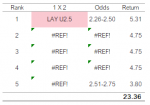
To find the return ive used a LARGE formula and that works fine,
To find the 1X2 column header i've used a INDEX & SUMPRODUCT with column*column formula
To find the Odds row header i've used the same as above but with the row*row formula

The problem arises when i have identical ( see below ) values the INDEX & SUMPRODUCT formulas do not return the relevant values

Can this be resolved using the formula already in place? or will i need to add a helper table to resolve, bear in mind this data changes when the slicer option is changed

Many Thanks

 

[KRice]

What version of Excel are you using? You should update your profile to include that information, as it can have a bearing on which solutions might work best for you.

Here is one idea, although I think it can be improved. This uses a helper table in AA7:AE24 that mirrors the size of your pivot table. The helper table holds sequential values...that is its only purpose. The idea is to make the logical comparisons (e.g., does V7:Z24=some value, and then multiply that resulting table of TRUE's and FALSE's by the sequential values in the helper table. If you have the SEQUENCE function (I do not) there may be a way to eliminate the helper table altogether. In any case, this operation results in a matrix whose values are either 0 or some positive integer that identifies the location in the matrix (since we know the number of columns and rows in that matrix). Then the CEILING and MOD functions are used to determine the row and column indexes, and when used in conjunction with the INDEX function, the row and column header details can be identified.

One thing that needs to be clarified...when there are multiple matches, in which order should the matches be reported? For example, in this case, the 5th largest value to find in the data table is 3.80. There are two matches, but since you want only the five largest values, only one of these 3.80 matches will be reported as the 5th data point. Which is it? The formula I've used (AGGREGATE with the 14 option) will return the largest values, and in this case that means the largest values found in the helper array, so values are reported in an order generally corresponding to a direction that starts at the lower right and moves toward the upper left. If you want a different order, then some further adjustments would be necessary.

Here is a snapshot using the XL2BB add-in that looks similar to what you've posted. It may facilitate others offering some improvements.

MrExcel20200708.xlsx
	J	K	L	M	N	O	P	Q	R	S	T	U	V	W	X	Y	Z	AA	AB	AC	AD	AE
6													LAY Home	LAY Draw	LAY Away	LAY U2.5	LAY O2.5
7												1.21-1.30						1	2	3	4	5
8												1.41-1.50						6	7	8	9	10
9												1.51-1.60						11	12	13	14	15
10												1.61-1.70	-1.40	-1.30	1.90	0.30	-0.55	16	17	18	19	20
11	1 X 2	Odds	Return									1.71-1.80	-1.44	3.80	-3.10	-2.96	3.80	21	22	23	24	25
12	LAY U2.5	2.26-2.50	5.31									1.81-1.90	-0.25	4.75	-8.38	-0.60	0.47	26	27	28	29	30
13	LAY Away	2.51-2.75	4.75									1.91-2.00	-0.81	-1.30	1.05	-2.05	1.66	31	32	33	34	35
14	LAY Draw	2.51-2.75	4.75									2.01-2.25	2.18	-2.90	-1.13	-2.67	2.09	36	37	38	39	40
15	LAY Draw	1.81-1.90	4.75									2.26-2.50	2.39	3.35	-7.02	5.31	-4.20	41	42	43	44	45
16	LAY O2.5	1.71-1.80	3.80									2.51-2.75	-4.89	4.75	4.75	-3.04	1.54	46	47	48	49	50
17												2.76-3.00	3.53	1.45	-1.42	2.95	-1.81	51	52	53	54	55
18												3.01-3.50	1.14	-1.95	2.28	0.60	-0.48	56	57	58	59	60
19												3.51-4.00	1.49	-5.55	2.61	0.10	-0.15	61	62	63	64	65
20												4.01-4.50	-0.30	0.95	0.95	0.95	-0.34	66	67	68	69	70
21																		71	72	73	74	75
22																		76	77	78	79	80
23																		81	82	83	84	85
24																		86	87	88	89	90
25
Sheet4

Cell Formulas
Range	Formula
AA7:AE24	AA7	=COLUMNS($V$6:V$6)+(ROWS($U$7:$U7)-1)*COLUMNS($V$6:$Z$6)
J12:J16	J12	=INDEX($V$6:$Z$6,,MOD(AGGREGATE(14,6,($V$7:$Z$24=$L12)*($AA$7:$AE$24),COUNTIF($L$12:$L12,$L12))-1,COLUMNS($V$6:$Z$6))+1)
K12:K16	K12	=INDEX($U$7:$U$24,CEILING(AGGREGATE(14,6,($V$7:$Z$24=$L12)*($AA$7:$AE$24),COUNTIF($L$12:$L12,$L12) )/COLUMNS($V$6:$Z$6),1))
L12:L16	L12	=LARGE($V$7:$Z$24,ROWS(L$12:L12))

 

[juca73]

KRice

Thank you so much, all of the above is working perfectly. ( using 365 & 2010 )
In answer to the 'when there are multiple matches, in which order should the matches be reported?' question, for this purpose in the rank 5th position it would be the duplicated value that appears first.

Nevertheless, you have saved me from continual headaches over this

 

[KRice]

You're welcome. I'm not quite sure that I follow your answer...the "duplicated value that appears first" part. If there are duplicate values, do you want them listed in order from upper left to lower right (which is the reverse of what I show)? Since you have 365, you might try replacing the references to the helper table...the *($AA$7:$AE$24) in the formulas with *SEQUENCE(ROWS($U$7:$U$24),COLUMNS($V$6:$Z$6),1,1)
I'm not able to confirm this, but I think that will give the same matrix as the helper table...in which case the helper table would not be necessary. You could try this for one of the results columns J or K, and if it works, do a similar substitution in the other formula.

If that works, then depending on the clarification to the order question, another adjustment might be needed.

 

[juca73]

I apologize, the order that you have done it is fine. i'll try the alternative formula and let you know if its successful...once again many many thanks