Help needed with the calculation/formula

[justme101]

Hello all,

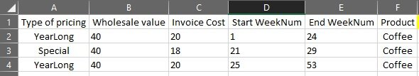
I have an excel file with 1000s of lines of products and cost details for them as well. Given below is a sample data:

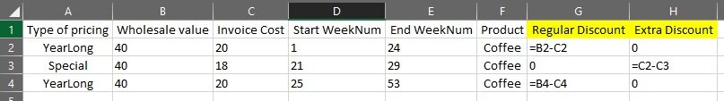
And what you see below has two added columns where I need help with the formula:

As you can see, the requirement "looks" pretty simple. If in column A, the type of pricing is YearLong, the calculation is to be done in column G (Regular discount), and the value should come as B2 - C2, which is $20 in this case and it runs from week 1 to week 24 of the year. From week 25, this pricing gets updated and we will be giving B4-C4, $40 - $22, $18 Regular discount.

The issue comes in row 3 when I have to calculate the extra discount. Whenever there is a type of pricing "Special" in column A, the calculation has to happen in column H (Extra discount). Since, the "start week" of the special discount is week 21, you can understand that from weeks 21 through 24 the extra discount should be - the YearLong invoice cost for these weeks (column C) minus the Invoice Cost for the Special price in these weeks, i.e. $20 - $18 = $2 should be coming for those weeks, and from weeks 25 onwards when the invoice cost for YearLong discount increases to $22, the special discount from weeks 25 - 53 will be $22 - $18 = $4. Hence, the final value in the Extra Discount column for this product should be the weighted average of these two blended pricing.

Looks simple if there are only 3 rows an only 1 product, but there are 1000s of lines like I said and manually doing this is a pain in the behind. I am open to formulas as well as macro solutions for this calcualtion. It will be a life saver if any of you can help out. Thank you.

 

[awoohaw]

I'm not sure why you have 3 rows for one product. Can't you have one row per product? What is it you do with the different values calculated on the 3 rows?
Or,
Why do you have to have two different discount calculations, why can''t you put a conditional statement in column G calculation to use the special pricing when it is present?

Also, if you use the xl2bb add in, or post as a table instead of posting photos the forum can help you better (they don't have to spend time recreating your data).

 

[justme101]

I'm not sure why you have 3 rows for one product. Can't you have one row per product? What is it you do with the different values calculated on the 3 rows?
Or,
Why do you have to have two different discount calculations, why can''t you put a conditional statement in column G calculation to use the special pricing when it is present?

Also, if you use the xl2bb add in, or post as a table instead of posting photos the forum can help you better (they don't have to spend time recreating your data).

Well, there will be multiple rows depending on when each type of pricing starts and stops. For e.g. if there is a new Special pricing from week 30 to 40, there will be a new row for it. That is how the base file is set and I cannot make changes to it.

To your second point, I am very open to getting the final calculation in a single column, no matter what type of pricing it is, but at this moment it is how the file is made up, and changing it will open up a lot of other issues, as there are several sheets linked to this one.

For the xl2bb add in, i did install it but not sure why it didn't work for me, i will try to do it again.

 

[awoohaw]

ok. If you can't install the add in, please post a table.

(did you go to FILE>>OPTIONS>>Add Ins, and add the add in?)

 

[Fluff]

For the xl2bb add in, i did install it but not sure why it didn't work for me, i will try to do it again.

Have a look here XL2BB Icons greyed out to see if it helps.

 

[justme101]

I

ok. If you can't install the add in, please post a table.

(did you go to FILE>>OPTIONS>>Add Ins, and add the add in?)

think I got it working now. Is this OK?

Book2.xlsx
	A	B	C	D	E	F	G	H
1	Type of pricing	Wholesale value	Invoice Cost	Start WeekNum	End WeekNum	Product	Regular Discount	Extra Discount
2	YearLong	$ 40.00	$ 20.00	1	24	Coffee	$ 20.00	$ -
3	Special	$ 40.00	$ 18.00	21	29	Coffee	$ -	$ 2.00
4	YearLong	$ 40.00	$ 22.00	25	53	Coffee	$ 18.00	$ -
Sheet1

Cell Formulas
Range	Formula
G2,G4	G2	=B2-C2
H3	H3	=C2-C3

 

[awoohaw]

Try this:
(But I think I am missing something)
(this requires that there is always a yearlong row before the special row, and only one special row)

Book1
	A	B	C	D	E	F	G	H	I
1	Type of pricing	Wholesale value	Invoice Cost	Start WeekNum	End WeekNum	Product	Regular Discount	Extra Discount	Discount:
2	YearLong	40	20	1	24	Coffee	20		20
3	Special	40	18	21	29	Coffee		2	2
4	YearLong	40	22	25	53	Coffee	18		18
justme101

Cell Formulas
Range	Formula
G2,G4	G2	=B2-C2
H3	H3	=C2-C3
I2:I4	I2	=IF(A2="Special",C1,B2)-C2