HELP! Sum rows that contain letters

[mesa]

Hello,

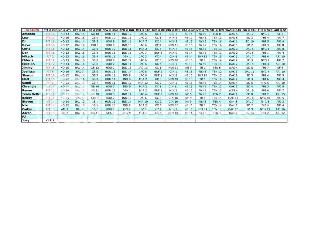
I run a football pick'em league and I need to find a way to sum rows that contain letters. So below is a jpg of my spreadsheet with the sum would come out to 136, but at times I make mistakes and enter the same number twice in a row. So if I had a formula that would sum the numbers in the row and the sum was different than 136 I can find where I made a mistake. The first row would sum the numbers through B2 to Q2 and equal 136. Thank in advance!

Example:

 

[Andrew Poulsom]

Try:

=SUMPRODUCT(--MID(B2:Q2,FIND(" ",B2:Q2)+1,255))

 

[mesa]

Try:

=SUMPRODUCT(--MID(B2:Q2,FIND(" ",B2:Q2)+1,255))

It works! Thank you so much.

Since I have you here... I have one more question. With this formula is there anyway it can be modified so when I change the font color to red it will not sum that box?

How I run my league is when a team losses I change the font color to red indicating that the team has lost and the person that picked them will not receive points. So in my example (B2 to Q2) above the total would come to 120 since PIT lost. So, Is there anyway the formula can be modified so when I change the font to red the point will not be calculated into the final product?

Again, THANK YOU so much. If this request can't be fulfilled I understand, you have done so much already! Thank you!

Steven

 

[mesa]

Bump

 

[Andrew Poulsom]

You can use Chip Pearson's CountColor function from here:

http://www.cpearson.com/Excel/colors.aspx

 

[mesa]

You can use Chip Pearson's CountColor function from here:

http://www.cpearson.com/Excel/colors.aspx

I don't have a clue how this stuff works ..lol. But thank you so much for the formula you wrote. I'll do my best to figure out the CountColor function and apply it to my spreadsheet/formula.

Thanks again!

 

[mesa]

Was hoping if someone could help me with this forumla =SUMPRODUCT(--MID(B2:Q2,FIND(" ",B2:Q2)+1,255)) to make it only sum black font or exclude red font. Either would be fine.

I tried using ColorIndexOfRange and CountColor operations to modifiy the above formula but with no luck. Not sure if I'm on the right track or not.

Thanks in advance!

 

[Dave Patton]

A quick thought.
If you put an "x" in front of the text of the losing team and possibly use conditional formatting to colour the cell, a formula building on Andrew's suggestion should work.

The following is an array formula, edit the ranges and enter the formula with Ctrl+Shift+Enter (CSE) not just Enter.

=SUM(IF(LEFT(B2:C2,1)<>"x",--MID(B2:C2,FIND(" ",B2:C2)+1,255)))

 

[mesa]

A quick thought.
If you put an "x" in front of the text of the losing team and possibly use conditional formatting to colour the cell, a formula building on Andrew's suggestion should work.

The following is an array formula, edit the ranges and enter the formula with Ctrl+Shift+Enter (CSE) not just Enter.

=SUM(IF(LEFT(B2:C2,1)<>"x",--MID(B2:C2,FIND(" ",B2:C2)+1,255)))

I might have to give that a try, but I really want to stay with just changing the font color -- it's what my members are used to. There seem to be a way to do this but reading the link above using the ColorCount function but just can't figure it out

 

[Andrew Poulsom]

This worked for me:

=SUMPRODUCT(--(ColorIndexOfRange(B2:Q2)<>3),--(MID(B2:Q2,FIND(" ",B2:Q2)+1,255)))