Help summarizing inventory spreadsheet

girkinz

New Member
Joined
Jan 27, 2023
Messages
3
Office Version
  1. 365
Platform
  1. Windows
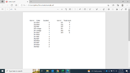
I'm brand new to using Excel and I am trying to summarize an inventory from a rather large source sheet. On the summary sheet, I used =UNIQUE(INVENTORY!B8:B47) to tell me all of the things we carry, and =SUMIF(INVENTORY!B8:B47, SUMMARY!B8#, INVENTORY!D8:D47) to display how many we have in stock. It's important to know how many we have of each color so I'm trying to find a way to list that. Preferrably the output of this function would just be a list of the colors we have and how many of that color we have in stock for each unique item we have. Everything we have comes in different colors so I'd hate to list them all and use the count function in the basic way that I know how. I've tried a few things but, obviously, none of them work!
 

Excel Facts

Pivot Table Drill Down
Double-click any number in a pivot table to create a new report showing all detail rows that make up that number
Welcome to the Board

Are you able to show a sample of data and expected results?

If you are simply counting, try using Countif, instead of sumif?
 
Upvote 0
Welcome to the Board

Are you able to show a sample of data and expected results?

If you are simply counting, try using Countif, instead of sumif?

Thanks for responding! This is kind of a simple example because it doesn't show how many color categories I actually have to account for. I've tried countif in the ways I know how, but I'm not sure how to avoid listing every color we have when not every color is applicable to every item. If there was something that could just come back with each applicable color and how many times it appears for each item that would be ideal!
 

Attachments

  • Screenshot (2).png
    Screenshot (2).png
    177.6 KB · Views: 7
Upvote 0
Having looked at the data you posted, it does look like the formula you are using works
Book1
ABCDEFG
1ItemColorStockedTotal stock
2331Blue53315
3332Blue23324
4332Red23373
5337Orange33117
6311Orange131212
7311Blue13146
8311Blue1
9311Red4
10312Red3
11312Blue3
12312Red6
13314Blue4
14314Red2
Sheet1
Cell Formulas
RangeFormula
E2:E7E2=UNIQUE(A2:A14)
F2:F7F2=SUMIF(A2:A14,E2#,C2:C14)
Dynamic array formulas.
 
Upvote 0

Forum statistics

Threads
1,215,701
Messages
6,126,297
Members
449,308
Latest member
VerifiedBleachersAttendee

We've detected that you are using an adblocker.

We have a great community of people providing Excel help here, but the hosting costs are enormous. You can help keep this site running by allowing ads on MrExcel.com.
Allow Ads at MrExcel

Which adblocker are you using?

Disable AdBlock

Follow these easy steps to disable AdBlock

1)Click on the icon in the browser’s toolbar.
2)Click on the icon in the browser’s toolbar.
2)Click on the "Pause on this site" option.
Go back

Disable AdBlock Plus

Follow these easy steps to disable AdBlock Plus

1)Click on the icon in the browser’s toolbar.
2)Click on the toggle to disable it for "mrexcel.com".
Go back

Disable uBlock Origin

Follow these easy steps to disable uBlock Origin

1)Click on the icon in the browser’s toolbar.
2)Click on the "Power" button.
3)Click on the "Refresh" button.
Go back

Disable uBlock

Follow these easy steps to disable uBlock

1)Click on the icon in the browser’s toolbar.
2)Click on the "Power" button.
3)Click on the "Refresh" button.
Go back
Back
Top