Highlight Adjacent Cells in a grid

JLEMS

New Member
Joined
May 27, 2020
Messages
16
Office Version
  1. 365
Platform
  1. Windows
Hi. I am new here and I have been trying to figure out how to get a spreadsheet to do what I need it to, but have not found the exact way to get it done. I have a 10X10 grid of random numbers. What I want to happen is I want a formula encompassing the entire grid, and highlight only the cells that are adjacent to each other if all 3 numbers are there. For example, I included a smaller scale image. I have a grid of numbers and only want the 312 to highlight, but only if the cells are adjacent to each other. I don't want it to highlight all the 3's 1's and 2's. Only if all 3 are there.

Think of it like a wordsearch puzzle. Does this make any sense and can anyone help?

Thanks
 

Attachments

  • 312.jpg
    312.jpg
    17.5 KB · Views: 9

Excel Facts

Move date out one month or year
Use =EDATE(A2,1) for one month later. Use EDATE(A2,12) for one year later.
We're creating a lottery tool that I use based on a grid. I basically want to put in the numbers from the previous draw, and I want it to highlight the cells but only if they touch each other. That last one was almost perfect, I think only 1 number was not highlighted that should have been. does that make sense? I currently have a similar thing, but it highlights ALL of the 3's, 2's, and 1's. I was hoping that a formula existed to narrow it down to only the sections that the numbers meet.
 
Upvote 0
In this grid the highlighted area is the only area 312 touches each other. Regardless of it being 123,132,231,213,312,321 that is the only area. Is this helping?
 

Attachments

  • Untitled.png
    Untitled.png
    10.6 KB · Views: 8
Upvote 0
Just to clarify, in your first image did you miss highlighting some cells?
It should be like that:

1590599215862.png
 
Upvote 0
I must have, My apologies. That what you have there looks like it worked exactly how I need it to
 
Upvote 0
I suggest you use the following macro. Capture your numbers on the grid and run this macro:

VBA Code:
Sub Highlight_Adjacent_Cells()
  Dim r As Range, b As Range, ncell As String
  Dim k As Long, h As Long, resto As String, sNums As Variant

  Application.ScreenUpdating = False
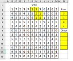
  Set r = Range("B2:M13")
  r.Interior.ColorIndex = xlNone
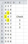
  sNums = Array([O3] & [O4] & [O5], [O3] & [O5] & [O4], [O5] & [O3] & [O4])
  For h = 0 To UBound(sNums)
    Set b = r.Find(Left(sNums(h), 1), , xlValues, xlWhole)
    If Not b Is Nothing Then
      ncell = b.Address
      Do
        For k = 1 To 8
          resto = Mid(sNums(h), 2, Len(sNums(h)))
          Call busca(r, resto, k, b.Row, b.Column, b)
        Next
        Set b = r.FindNext(b)
      Loop While Not b Is Nothing And b.Address <> ncell
    End If
  Next
  Application.ScreenUpdating = True
End Sub

Sub busca(r, resto, k, f, c, b)
  Dim i As Long, j As Long, n As Long, m As Long
  Select Case k
    Case 1: f = f - 1: c = c + 0
    Case 2: f = f - 1: c = c + 1
    Case 3: f = f + 0: c = c + 1
    Case 4: f = f + 1: c = c + 1
    Case 5: f = f + 1: c = c + 0
    Case 6: f = f + 1: c = c - 1
    Case 7: f = f + 0: c = c - 1
    Case 8: f = f - 1: c = c - 1
  End Select
  
  If f >= r.Rows(1).Row And f <= r.Rows(r.Rows.Count).Row _
    And c >= r.Columns(1).Column And c <= r.Columns(r.Columns.Count).Column Then
    If Cells(f, c) = Val(Mid(resto, 1, 1)) Then
      For i = 2 To Len(resto)
        For n = 1 To 8
          Select Case n
            Case 1: j = f - 1: m = c + 0
            Case 2: j = f - 1: m = c + 1
            Case 3: j = f + 0: m = c + 1
            Case 4: j = f + 1: m = c + 1
            Case 5: j = f + 1: m = c + 0
            Case 6: j = f + 1: m = c - 1
            Case 7: j = f + 0: m = c - 1
            Case 8: j = f - 1: m = c - 1
          End Select
          If j >= r.Rows(1).Row And j <= r.Rows(r.Rows.Count).Row _
            And m >= r.Columns(1).Column And m <= r.Columns(r.Columns.Count).Column Then
            If Cells(j, m) = Val(Mid(resto, i, 1)) Then
              b.Interior.ColorIndex = 6
              Cells(f, c).Interior.ColorIndex = 6
              Cells(j, m).Interior.ColorIndex = 6
            End If
          End If
        Next n
      Next i
    End If
  End If
End Sub

Considerations:
1. It works only for 3 numbers.
2. The numbers must be one digit.
1590608146347.png


__________________________________________________________________________________________________________
It is a very long macro, maybe there is a more simplified way, hopefully someone can help us.
 
Upvote 0
It is a long macro, and it seems to work exactly how I want it to. Is there a simplified way to do this? Is there a conditional formatting for this that would not require a Macro?
 
Upvote 0
Mark, I'll see if I can come up with some ideas on that:coffee: But I assume it is not easy to do that with conditional formatting, a Macro is the best way for now.
 
Upvote 0
it seems to work exactly how I want it to
For now, you could work with that, let me know if any combination of numbers is not highlighted.

__________________________________________________________________________________________________________________
Is there a simplified way to do this?
Recursion is not a simple topic, or at least for me it is not simple, but I'll see if I can improve the macro.
 
Upvote 0
I think I made it using conditional formatting. Ignore the different colors, i use different colors to check formulas.
OR=={-2,-2,-2;-1,-1,-1;0,0,0}
OC=={-2,-1,0;-2,-1,0;-2,-1,0}


Cell Formulas
RangeFormula
D7:M16D7=RANDBETWEEN(0,9)
Cells with Conditional Formatting
CellConditionCell FormatStop If True
D7:M16Expression=OR(D7=1,D7=2,D7=3)*COUNT(0/COUNTIF(OFFSET(D7,-1,-1,3,3),ROW($1:$3)))=3textNO
D7:M16Expression=(D7=3)*OR((OFFSET(D7,-1,-1,3,3)=2)*COUNTIF(OFFSET(D7,OR,OC,3,3),1))textNO
D7:M16Expression=(D7=3)*OR((OFFSET(D7,-1,-1,3,3)=1)*COUNTIF(OFFSET(D7,OR,OC,3,3),2))textNO
D7:M16Expression=(D7=2)*OR((OFFSET(D7,-1,-1,3,3)=3)*COUNTIF(OFFSET(D7,OR,OC,3,3),1))textNO
D7:M16Expression=(D7=2)*OR((OFFSET(D7,-1,-1,3,3)=1)*COUNTIF(OFFSET(D7,OR,OC,3,3),3))textNO
D7:M16Expression=(D7=1)*OR((OFFSET(D7,-1,-1,3,3)=3)*COUNTIF(OFFSET(D7,OR,OC,3,3),2))textNO
D7:M16Expression=(D7=1)*OR((OFFSET(D7,-1,-1,3,3)=2)*COUNTIF(OFFSET(D7,OR,OC,3,3),3))textNO
 
Last edited by a moderator:
Upvote 0

Forum statistics

Threads
1,214,983
Messages
6,122,591
Members
449,089
Latest member
Motoracer88

We've detected that you are using an adblocker.

We have a great community of people providing Excel help here, but the hosting costs are enormous. You can help keep this site running by allowing ads on MrExcel.com.
Allow Ads at MrExcel

Which adblocker are you using?

Disable AdBlock

Follow these easy steps to disable AdBlock

1)Click on the icon in the browser’s toolbar.
2)Click on the icon in the browser’s toolbar.
2)Click on the "Pause on this site" option.
Go back

Disable AdBlock Plus

Follow these easy steps to disable AdBlock Plus

1)Click on the icon in the browser’s toolbar.
2)Click on the toggle to disable it for "mrexcel.com".
Go back

Disable uBlock Origin

Follow these easy steps to disable uBlock Origin

1)Click on the icon in the browser’s toolbar.
2)Click on the "Power" button.
3)Click on the "Refresh" button.
Go back

Disable uBlock

Follow these easy steps to disable uBlock

1)Click on the icon in the browser’s toolbar.
2)Click on the "Power" button.
3)Click on the "Refresh" button.
Go back
Back
Top