Highlight coordinates / positions

[leturc]

Hi everybody,
I hope this message finds you well. I
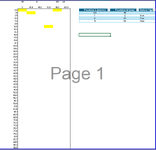
In my current project, I am working with a main table in Excel that represents fabric measurements. Specifically, the A column denotes the length, ranging from 1 to 100 meters (each row representing 1 meter), while the first row indicates the width, spanning from 0 to 150 cm (with 5 columns of 30 cm each).
Additionally, I maintain a separate defect table within the same Excel file. This defect table contains information about various defects found in the fabric, including the defect name, the meter at which it is present, and its position from the left selvage.
I need to highlight corresponding cell in the main table (surely between the range) based on the defect information stored in the defect table.
Could you kindly provide guidance or assistance on how to achieve this in Excel? Any insights or recommendations would be greatly appreciated.
Thank you for your time and support.

 

[DanteAmor]

Use the following conditional formatting.

Create a new rule in conditional formatting and add the formula at the bottom of the example.

Before you must add a larger number to your measurements, in cell H3 I added 200 and in cell A52 I added 100. This is for the purposes of the formula. You must do it in the cells of your sheet.

Unfortunately, the rows and columns of your sheet are not visible in your image, so you will have to adapt the formula and the range to where you want it to work.

varios 21mar2024.xlsm
	A	B	C	D	E	F	G	H	I	J	K
1		88	m			120	cm
2
3		0.0	24.0	48.0	72.0	96.0	120.0	200.0	Position L	Position W	Defect
4	0.0								0.5	110
5	1.8								1	2	K
6	5.3								2	44	T
7	7.0								11	80	H
8	8.8
9	10.6
10	12.3
11	14.1
49	80.6
50	82.3
51	86.2
52	100.0
Hoja1

Cells with Conditional Formatting
Cell	Condition		Cell Format	Stop If True
B4:G52	Expression	=SUMPRODUCT((B$3<=$J$4:$J$7)*(C$3>$J$4:$J$7)*($A4<=$I$4:$I$7)*($A5>$I$4:$I$7))	text	NO

 

[leturc]

Use the following conditional formatting.

Create a new rule in conditional formatting and add the formula at the bottom of the example.

Before you must add a larger number to your measurements, in cell H3 I added 200 and in cell A52 I added 100. This is for the purposes of the formula. You must do it in the cells of your sheet.

Unfortunately, the rows and columns of your sheet are not visible in your image, so you will have to adapt the formula and the range to where you want it to work.

varios 21mar2024.xlsm
	A	B	C	D	E	F	G	H	I	J	K
1		88	m			120	cm
2
3		0.0	24.0	48.0	72.0	96.0	120.0	200.0	Position L	Position W	Defect
4	0.0								0.5	110
5	1.8								1	2	K
6	5.3								2	44	T
7	7.0								11	80	H
8	8.8
9	10.6
10	12.3
11	14.1
49	80.6
50	82.3
51	86.2
52	100.0
Hoja1

Cells with Conditional Formatting
Cell	Condition		Cell Format	Stop If True
B4:G52	Expression	=SUMPRODUCT((B$3<=$J$4:$J$7)*(C$3>$J$4:$J$7)*($A4<=$I$4:$I$7)*($A5>$I$4:$I$7))	text	NO

Dear DanteAmor,

Thnak you very vey much. It is working perfectly.