Highlight rows if values in a column are consecutive

Ofsthun01

New Member
Joined
Jul 31, 2021
Messages
12
Office Version
  1. 365
Platform
  1. Windows
Hello,

I'm trying to highlight all rows based on whether values in a certain column are consecutive numbers.

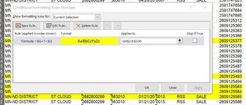
My spreadsheet is thousands of rows long and each cell in column I contains an 11-digit number. If any of those numbers are consecutive, I would like the whole row highlighted.

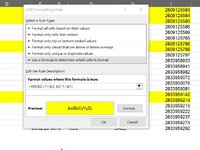
I tried this with conditional formatting with a basic =A2+1=A3 for example, and it wasn't highlighting properly. I have some VBA experience so if that's the needed route, no problem.

Thanks in advance!
Aaron
 

Excel Facts

Remove leading & trailing spaces
Save as CSV to remove all leading and trailing spaces. It is faster than using TRIM().
can you use a sample and XL2BB to show the sheet
=A2+1=A3 Should work,
But what does it wasn't highlighting properly.
mean

if you select a range A2:Z100 say
and your comparing column I

then formula would be I2+1=I3
need to add a $ to stop it moving and highlight the row
$I2+1=$I3

If you are selecting a range using the columns completely
then you need to use row 1
$I1+1=$I2

Note the Row number in the formula must match with the selection for conditional formatting

but you may need an OR()

=OR($I2+1=$I3, $I2-1=$I1), to get all values highlighted

Book1
ABCDEFGHIJKLMNO
21
32
44
56
67
78
89
90
Sheet1
Cells with Conditional Formatting
CellConditionCell FormatStop If True
A2:O9Expression=OR($I2+1=$I3, $I2-1=$I1)textNO
 
Upvote 0
Solution
So I want the formula to take the whole 11 digits into account, and it doesn't seem to be doing that. In the attachment, you can see it highlighted
2609125377 but not 2609125378. Or 2609125493 but not 2609125494.

Maybe I didn't explain what I want clearly enough, or I'm doing something wrong, sorry about that.

But I need the whole row highlighted for consecutive numbers that takes the whole value into account, not just the last digit.
So in the case of 2609125377 & 2609125378, I would want both rows highlighted. And I just can't seem to be able to get that to work.

Thank you for your reply
 

Attachments

  • screenshot.jpg
    screenshot.jpg
    152.7 KB · Views: 19
Upvote 0
You haven't used the right formula, you need this
Excel Formula:
=OR($I2+1=$I3, $I2-1=$I1)
 
Upvote 0
can you use a sample and XL2BB to show the sheet
=A2+1=A3 Should work,

mean

if you select a range A2:Z100 say
and your comparing column I

then formula would be I2+1=I3
need to add a $ to stop it moving and highlight the row
$I2+1=$I3

If you are selecting a range using the columns completely
then you need to use row 1
$I1+1=$I2

Note the Row number in the formula must match with the selection for conditional formatting

but you may need an OR()

=OR($I2+1=$I3, $I2-1=$I1), to get all values highlighted
Also, if i use the OR operator like you mentioned above, it still misses consecutive numbers, or highlights items which aren't consecutive at all. I don't understand what I'm missing. And thanks again for your help
 

Attachments

  • SharedScreenshot2.jpg
    SharedScreenshot2.jpg
    129.3 KB · Views: 32
Upvote 0
You haven't used the right formula, you need this
Excel Formula:
=OR($I2+1=$I3, $I2-1=$I1)
That formula also doesn't seem to work for my purpose. It's highlighting items which are not consecutive, or missing ones that are.
 

Attachments

  • SharedScreenshot2.jpg
    SharedScreenshot2.jpg
    129.3 KB · Views: 28
Upvote 0
what range did you select before applying the formatting ?
 
Upvote 0
what range did you select before applying the formatting ?
I may have selected the whole sheet. Now I selected column I and seems to work. I feel pretty stupid.Thank you for walking me through thi, sorry for the trouble.
 
Upvote 0
you are welcome
the selected are is important for the formatting to work based on formula

in my example i selected the sheet a to o , but the row 2 was selected and reference in formula
 
Upvote 0

Forum statistics

Threads
1,215,429
Messages
6,124,839
Members
449,193
Latest member
MikeVol

We've detected that you are using an adblocker.

We have a great community of people providing Excel help here, but the hosting costs are enormous. You can help keep this site running by allowing ads on MrExcel.com.
Allow Ads at MrExcel

Which adblocker are you using?

Disable AdBlock

Follow these easy steps to disable AdBlock

1)Click on the icon in the browser’s toolbar.
2)Click on the icon in the browser’s toolbar.
2)Click on the "Pause on this site" option.
Go back

Disable AdBlock Plus

Follow these easy steps to disable AdBlock Plus

1)Click on the icon in the browser’s toolbar.
2)Click on the toggle to disable it for "mrexcel.com".
Go back

Disable uBlock Origin

Follow these easy steps to disable uBlock Origin

1)Click on the icon in the browser’s toolbar.
2)Click on the "Power" button.
3)Click on the "Refresh" button.
Go back

Disable uBlock

Follow these easy steps to disable uBlock

1)Click on the icon in the browser’s toolbar.
2)Click on the "Power" button.
3)Click on the "Refresh" button.
Go back
Back
Top