Highlight times that are equal to or later than

[alexfooty]

I will do my best to try to explain my problem.

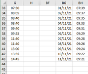
In Col G I have a list of times (hh:mm) that vary each day and also the number of rows may vary.
In Col BG I have a list of dates with a corresponding time in Col BH.

I would like to highlight any times in col G that are equal to, or later than, the time corresponding to today’s date in Col BH

In the following example, If today’s date was 05/11/2021, the corresponding time in Col BH would be 09:31. So any times equal to or later than that would be highlighted in Col G

I hope someone understands this - any help would be greatly appreciated.

 

[etaf]

try
a conditional formatting rule of
Select G2:G1000 - or however many rows likely to be

=G2>=(INDEX($BG$2:$BG$1000,MATCH(TODAY(),$BH$2:$BH$1000,0)))

heres an example using different columns for ease and smaller - so you just adjust the rows to match your data

Book7
	A	B	C	D
1
2	7:31		10/30/21
3	7:50		10/31/21
4	8:09		11/1/21	11:00
5	8:28		11/2/21	9:00
6	8:47
7	9:06
8	9:25
9	9:44
10	10:03
11	10:22
12	10:41
13	11:00
14	11:19
15	11:38
16	11:57
17	12:16
18	12:35
19	12:54
20	13:13
21	13:32
Sheet1

Cells with Conditional Formatting
Cell	Condition		Cell Format	Stop If True
A2:A21	Expression	=A2>=(INDEX($D$2:$D$5,MATCH(TODAY(),$C$2:$C$5,0)))	text	NO

 

[alexfooty]

Thanks etaf for your quick reply.
I used the conditional format formula you supplied but for some reason it isn't working.
Then I tried using the same setup as in your example - using Cols A,D & C and still not working.

It's possibly some stupid mistake on my behalf but I can't spot anything.

 

[etaf]

break it down in a other columns
its possible the times or dates are not real times or dates and just text
see what time just the index formula is returning

change the format of the cells to general and see if all the times and dates change to a number

not sure if xl2bb will show that
put column F I used
=INDEX($D$2:$D$5,MATCH(TODAY(),$C$2:$C$5,0))

dates are a number counting from 1900 , so 2nd Nov 2021 is the number 44502, and time is a decimal part of 1 so 12:00 is 0.5

Book7
	A	B	C	D	E	F
1						INDEX
2	0.31319444		44499			0.375
3	0.32638889		44500			0.375
4	0.33958333		44501	0.45833333		0.375
5	0.35277778		44502	0.375		0.375
6	0.36597222					0.375
7	0.37916667					0.375
8	0.39236111					0.375
9	0.40555556					0.375
10	0.41875					0.375
11	0.43194444					0.375
12	0.44513889					0.375
13	0.45833333					0.375
14	0.47152778					0.375
15	0.48472222					0.375
16	0.49791667					0.375
17	0.51111111					0.375
18	0.52430556					0.375
19	0.5375					0.375
20	0.55069444					0.375
21	0.56388889					0.375
22						0.375
Sheet1

Cell Formulas
Range	Formula
F2:F22	F2	=INDEX($D$2:$D$5,MATCH(TODAY(),$C$2:$C$5,0))

Cells with Conditional Formatting
Cell	Condition		Cell Format	Stop If True
A2:A21	Expression	=A2>=(INDEX($D$2:$D$5,MATCH(TODAY(),$C$2:$C$5,0)))	text	NO

 

[alexfooty]

All the cells were correct format - times hh:mm, dates as dates.
Changed format to general and added the INDEX to Col F using formula.

Cols D & F did not change to a number but still showed as times (all cols format is general)

 

[etaf]

thats the issue column D is text and not a number / time , which is why its not working
column D needs to be time and change to a decimal of 1 like column A

you may be able to change the format of D by clicking on the column and DATA>text to columns >finish

 

[alexfooty]

Now that works perfectly - (can't say I follow whats going on but it works)
Do I just change col A back to hh:mm as that is the format I require?

 

[etaf]

yes, change the format as required
not sure which bit you are referring to as

(can't say I follow whats going on but it works)

The index/match

That is looking down the dates column and trying to match with a row where the date is today()
MATCH(TODAY(),$C$2:$C$5,0)
today() returns today's date and its looking down column C until it finds the row with the first matching date
then
INDEX($D$2:$D$5
is returning the same row but from the column D

Time is a fraction of 1 so you can treat it as a normal number

The index/match has returned the time , as i say which is decimal part of the number - so if 12:00 then 0.5 is returned by the index match

then A2 > = index
now its looking to see if a2 is greater than or equal to 0.5

With conditional formatting , think of it as a program that steps through each cell and checks if true or false

you have selected say A2 to A10
then added the formula
so conditional formatting will first check if A2 meets the criteria - TRUE/FALSE , if True then does whatever you format told it to do
IF you had STOP IF TRUE _ ticked in the conditional format then if it was TRUE , it would stop there
Then it checks A3 , A4, A5 etc and highlights all the cells that meet the criteria

Hope that helps a little

 

[alexfooty]

Hi etaf
Spreadsheet now up and functioning perfectly and the Index/Match explanation was extremely useful.
Thank you so much for all your help and undoubted patience - it is greatly appreciated.

 

[etaf]

you are welcome