highlighting cells with no value if they are between cells with value

[apor]

Hello everyone,

I am currently analzying scanning data in a warehouse. The purpose is to find out which days a certain product was not scanned and to highlight it.

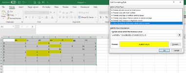
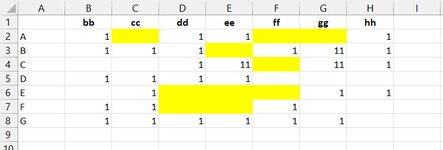
The data i am working with is a list of every product scanned and the day on which it was scanned. Then, I used a Pivot Table with y axis product and x axis day. If product A was scanned once on Monday, the field (Product, Day) has a 1. If it was scanned twice, a 2 and so on. I want to highlight the days it was not scanned at all.

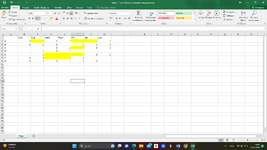
I added an image of how i would like the cells highlighted. The added complication in this case is that i cannot simply highlight blank cells, since for example, Product C was not introduced until Wednesday and it is therefore not a mistake that it was not scanned before then. Same goes with for example product F after Friday, since that was the last day it was there.

Any help with this would be greatly appreciated.

Thanks in advance and greeting,

Anna

 

[Anthony47]

Try using conditional format:
-select B2:CCxx where CC means "enough columns" and xx means enough rows
-apply a conditional format, using the following formula: =AND(B2="",SUM($B2:B2)>0,SUM(B2:$CC2)>0) In this formula "CC" means the last column selected

 

[apor]

Try using conditional format:
-select B2:CCxx where CC means "enough columns" and xx means enough rows
-apply a conditional format, using the following formula: =AND(B2="",SUM($B2:B2)>0,SUM(B2:$CC2)>0) In this formula "CC" means the last column selected

Hello Anthony, thank you for your response. Unfortunately, i get an error message when i enter this formula. is there maybe a syntax error i do not see?

 

[Anthony47]

How did you procede? Which formula did you use?

 

[apor]

Hello Anthony,

I used

=AND(B2="",SUM($B2:B2)>0,SUM(B2:$H2)>0)

I replaced CC with H and used your table that you sent. However, nothing gets highlighted, even though i used a color for the formatting and deleted all old rules before entering this one.

I also tried this formula as an example =AND($B2>5, $B2<20) and this does not highlight any cells for me either. =$B2<>10 for exmaple does though.

 

[apor]

This is what he formula loos like if i go back to edit it

 

[Anthony47]

That is a string, not a formula. Also AND is And, and SUM is Sum in your local language? And the field separator is comma (,) or semicolon (?

 

[Anthony47]

Maybe

=UND(B2="";SUMME($B2:B2)>0;SUMME(B2:$CC2)>0)

Translator

Lo strumento online per la traduzione di formule e funzioni di Excel da una lingua all'altra. Supporta la sostituzione dei separatori di argomenti, 35 lingue e molto altro ancora.

it.excel-translator.de

 

[apor]

Maybe

=UND(B2="";SUMME($B2:B2)>0;SUMME(B2:$CC2)>0)

Translator

Lo strumento online per la traduzione di formule e funzioni di Excel da una lingua all'altra. Supporta la sostituzione dei separatori di argomenti, 35 lingue e molto altro ancora.

it.excel-translator.de

i changed my language to english and i got a reaction out of the string

However, this is the result i get

 

[Anthony47]

I am afraid that you selected the wrong area when you setup the conditional format.
That formula is valid if you select from B2 to the end of your table; if the selected area at the moment is different you will get wrong results
So, my suggestion:
-remove the current conditional format rules
-select B2:XXyy
-apply the conditional format using the given formula