highlighting cells with no value if they are between cells with value

apor

New Member
Joined
Dec 20, 2021
Messages
25
Office Version
  1. 2016
Platform
  1. Windows
Hello everyone,

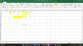
I am currently analzying scanning data in a warehouse. The purpose is to find out which days a certain product was not scanned and to highlight it.

The data i am working with is a list of every product scanned and the day on which it was scanned. Then, I used a Pivot Table with y axis product and x axis day. If product A was scanned once on Monday, the field (Product, Day) has a 1. If it was scanned twice, a 2 and so on. I want to highlight the days it was not scanned at all.

I added an image of how i would like the cells highlighted. The added complication in this case is that i cannot simply highlight blank cells, since for example, Product C was not introduced until Wednesday and it is therefore not a mistake that it was not scanned before then. Same goes with for example product F after Friday, since that was the last day it was there.

Any help with this would be greatly appreciated.

Thanks in advance and greeting,

Anna
 

Attachments

  • Screenshot (2).png
    Screenshot (2).png
    155 KB · Views: 9
I am afraid that you selected the wrong area when you setup the conditional format.
That formula is valid if you select from B2 to the end of your table; if the selected area at the moment is different you will get wrong results
So, my suggestion:
-remove the current conditional format rules
-select B2:XXyy
-apply the conditional format using the given formula
Thank you so much for your time! This worked perfectly :)
 
Upvote 0

Excel Facts

How can you turn a range sideways?
Copy the range. Select a blank cell. Right-click, Paste Special, then choose Transpose.
I am afraid that you selected the wrong area when you setup the conditional format.
That formula is valid if you select from B2 to the end of your table; if the selected area at the moment is different you will get wrong results
So, my suggestion:
-remove the current conditional format rules
-select B2:XXyy
-apply the conditional format using the given formula
If you have the time, could you give me a breakdown of what the string means? AND i know returns values if a condition is met, and then three conditions are stated

B2: "" means the cell has to be empty
however, what exactly do the SUM strings mean and how do they work together? and how does the string work throughout all cells of the table, not just B2 which is stated? is that due to CC2, which defines the last selected column? or because strings in conditional formatting "loop"?
 
Upvote 0
Excel Formula:
=AND(B2="",SUM($B2:B2)>0,SUM(B2:$CC2)>0)
The key is the type of absolute/relative addressing, and let's examine how it works on cell D3
When all
-"D3" is empty
-D2:D3 contains some values (the product has already been scanned in the past...)
-D3:CC3 contains some value (... and has some scanning in the future)
then the color will be applied to the cell

In other words, $B2 means "from column B of the current row; B2 when copied in eanche of the selected cells become "the current cell"; $CC means "up to column CC of the current row"
That's why it is important which area is selected when you set the conditional format

If that resolve the problem then it'd be better to mark the discussion as Resoved; see the procedure: Mark as Solution
 
Upvote 0
Solution

Forum statistics

Threads
1,215,093
Messages
6,123,068
Members
449,091
Latest member
remmuS24

We've detected that you are using an adblocker.

We have a great community of people providing Excel help here, but the hosting costs are enormous. You can help keep this site running by allowing ads on MrExcel.com.
Allow Ads at MrExcel

Which adblocker are you using?

Disable AdBlock

Follow these easy steps to disable AdBlock

1)Click on the icon in the browser’s toolbar.
2)Click on the icon in the browser’s toolbar.
2)Click on the "Pause on this site" option.
Go back

Disable AdBlock Plus

Follow these easy steps to disable AdBlock Plus

1)Click on the icon in the browser’s toolbar.
2)Click on the toggle to disable it for "mrexcel.com".
Go back

Disable uBlock Origin

Follow these easy steps to disable uBlock Origin

1)Click on the icon in the browser’s toolbar.
2)Click on the "Power" button.
3)Click on the "Refresh" button.
Go back

Disable uBlock

Follow these easy steps to disable uBlock

1)Click on the icon in the browser’s toolbar.
2)Click on the "Power" button.
3)Click on the "Refresh" button.
Go back
Back
Top