Hlookup 2nd instance trouble

[janderson055]

I'm fairly new to using excel and have been trying to create a simple spreadsheet that keeps track of scores and automatically displays the names of the players in descending order. Anyway I have gotten to the point of using hookup to match a value and return that players name. But when two players have the same score it will only return the first found value. I sort the number scores using a LARGE function and it works great. Then I use something like this =HLOOKUP(Y2,B27:K28,2,FALSE) to match that value with the players name. Any suggestions on how to return the other players name when the scores are the same?

 

[T. Valko]

I'm fairly new to using excel and have been trying to create a simple spreadsheet that keeps track of scores and automatically displays the names of the players in descending order. Anyway I have gotten to the point of using hookup to match a value and return that players name. But when two players have the same score it will only return the first found value. I sort the number scores using a LARGE function and it works great. Then I use something like this =HLOOKUP(Y2,B27:K28,2,FALSE) to match that value with the players name. Any suggestions on how to return the other players name when the scores are the same?

Can you post some sample data so we can see what you're looking for?

I understand what you want to do but need to see how the data is setup to be able to make a suggestion.

 

[janderson055]

 

[T. Valko]

...

OK, let's assume you have the scores listed starting in Y2 in descending order.

Book1
	Y	Z
2	2150	Player5
3	1800	Player8
4	1700	Player4
5	1550	Player10
6	1300	Player7
7	1300	Player9
8	1100	Player6
9	1000	Player3
10	800	Player2
11	700	Player1
Sheet1

Enter this array formula** in Z2 and copy down as needed:

=INDEX($28:$28,SMALL(IF(B$27:K$27=Y2,COLUMN(B27:K27)),COUNTIF(Y$2:Y2,Y2)))

** array formulas need to be entered using the key
combination of CTRL,SHIFT,ENTER (not just ENTER).
Hold down both the CTRL key and the SHIFT key
then hit ENTER.

 

[janderson055]

That works awesome. Flawless. Thanks so much for the speedy response. You guys are geniuses.

 

[T. Valko]

That works awesome. Flawless. Thanks so much for the speedy response. You guys are geniuses.

You're welcome. Thanks for the feedback!

 

[janderson055]

No problem. I was also just wondering how that function works. I've used the IF and COUNTIF functions before, but never used the INDEX function before. If it isn't too much trouble can you please explain it a bit to me so I can use it later if need be. Thanks.

 

[T. Valko]

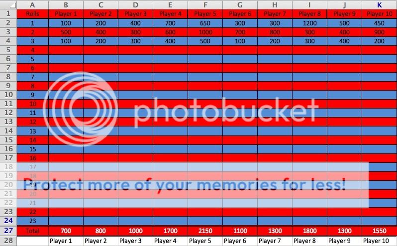
No problem. I was also just wondering how that function works. I've used the IF and COUNTIF functions before, but never used the INDEX function before. If it isn't too much trouble can you please explain it a bit to me so I can use it later if need be. Thanks.

Let's look at this smaller example:

Book1
	A	B	C	D	E	F
1	Name	Player1	Player2	Player3	Player4	Player5
2	Score	100	200	100	300	200
Sheet1

Book1
	A	B
5	Score	Name
6	300	Player4
7	200	Player2
8	200	Player5
9	100	Player1
10	100	Player3
Sheet1

This array formula** entered in B6 and copied down:

=INDEX($1:$1,SMALL(IF(B$2:F$2=A6,COLUMN(B2:F2)),COUNTIF(A$6:A6,A6)))

** array formulas need to be entered using the key
combination of CTRL,SHIFT,ENTER (not just ENTER).
Hold down both the CTRL key and the SHIFT key
then hit ENTER.

Here's how that formula works...

Look in this range (row 1) for the data we want to extract:

INDEX($1:$1

Each cell that is indexed is stored as a relative position. The positions start from 1 to the total number of cells in the indexed range. Depending on what version of Excel you're using if we index all of row 1 then the positions are:

In Excel 2007 and later: 1 to 16384

In Excel 2003 and earlier: 1 to 256

A1 = position 1
B1 = position 2
C1 = position 3
D1 = position 4
etc
etc

If we index the range D1:G1 then:

D1 = position 1
E1 = position 2
F1 = position 3
G1 = position 4

Now we need to tell the INDEX function we want to extract the data from the cells (positions) that meet a certain condition. In this case the condition is the player names that correspond to the nth largest numeric value from the range B2:F2.

We have the numeric values (scores) listed in descending order starting in cell A6.

We use this expression to return an array of the column numbers of the cell(s) that hold the nth largest score. If a cell does not contain the score we're looking for then the expression returns FALSE.

IF(B$2:F$2=A6,COLUMN(B2:F2))

For A6 (score 300) the array would look like this:

{FALSE,FALSE,FALSE,5,FALSE}

That tells us the score 300 was found in column number 5.

This array is passed to the SMALL function:

SMALL({FALSE,FALSE,FALSE,5,FALSE},

Then we have to tell the SMALL function which numeric value to pass to the INDEX function to exctract the data we want. We do that with the COUNTIF function.

When a score is unique then there will only be 1 column number in the array but when there are duplicate scores then there will be multiple column numbers in the array. For example, for score 200 the array would look like this:

{FALSE,3,FALSE,FALSE,6}

As the formula is entered and copied down the COUNTIF function will return the count of how many times the score appears in the range. We use this count to pass the nth smallest column number from the array to the INDEX function as the position number for the data we want to extract.

So, for A6 (score 300):

=INDEX($1:$1,SMALL({FALSE,FALSE,FALSE,5,FALSE},1))
=INDEX($1:$1,5)

Return the value from positon 5 of the indexed range (row 1). Positon 5 = cell E1 = Player 4.

For A7 (score 200):

=INDEX($1:$1,SMALL({FALSE,3,FALSE,FALSE,6},1))
=INDEX($1:$1,3)

Return the value from positon 3 of the indexed range (row 1). Positon 3 = cell C1 = Player 2.

For A8 (score 200 duplicate):

=INDEX($1:$1,SMALL({FALSE,3,FALSE,FALSE,6},2))
=INDEX($1:$1,6)

Return the value from positon 6 of the indexed range (row 1). Positon 6 = cell F1 = Player 5.

etc
etc
etc