How does one collate dates into Monday-Sunday ranges and sum up the data in 2nd Column to those date ranges

[Rhothgar]

I am sure there will be a simple answer to this but I've been trying to research how to do this and have scratched my head for hours.

I know it's not Get Data>Combine Queries>Merge!

I have a dataset? called TSS and a date range (UK format - DD/MM/YYYY) of 01/01/2021 (This was a Friday) - 31/12/2021 (Also a Friday perchance!)

I would like to be able to quickly collate:-

01/01/2021 - 03/01/2021 then,
04/01/2021 - 10/01/2021 then
11/01/2021 - 17/01/2021 and so on and so forth but ending with
20/12/2021 - 26/12/2021 and
27/12/2021 - 31/12/2021

Technically, if this is too difficult I would be able to add in the preceding days before 01/01/2021 to make a full week's data and 01/01/2022 and 02/01/2022 to make a full week at the year end if it makes the job easier.

Then the data in the TSS column would need to sum up for those date ranges so I have the weekly TSS total.

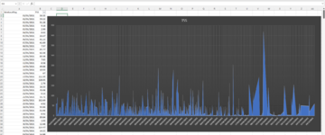
I have created a basic chart. Ultimately, I would then like to compare it to 2022 data on the same graph so I can see whether more work was done in either year on any given week.

I attach a screenshot of part of the data to give a clearer idea of where I am. Obviously the screenshot shows individual days at present in terms of TSS not having been collated. It can even be in a bar chart format. I am not particularly concerned with how it looks if the chart I have chosen cannot handle what I am trying to achieve.

I have absolutely no idea about VBA or coding or whether that would be needed to achieve what I would like to see. I am only a basic Excel user unlike many of you incredibly clever bods!

 

[Dave Patton]

"The formula is total gobbledy-gook to me but what is the difference between your C2 and D2 formulas as they appear achieve the same result? Is it just another way of achieving what C2 does so that either could be used. I do not appear to need both."
The C and D are alternatives; choose the formula that you prefer. The Sumifs may be more efficient.
To help understand formulas and to help build formulas, try Excel's Formulas Formula Evaluate.

To have data to chart consider the following.

SumProduct 2022a.xlsm
	G	H
1		Sum by week
2	Sun 3-Jan-21	220.47
3	Sun 10-Jan-21	193.22
4	Sun 17-Jan-21	350.00
5	Sun 24-Jan-21	145.00
6	Sun 31-Jan-21	0.00
2b

Cell Formulas
Range	Formula
H2:H6	H2	=SUMIFS(B:B,A:A,"<="&G2,A:A,">="&G2-6)

Named Ranges
Name	Refers To	Cells
Dates	='2b'!$A$2:$A$22	H2:H6
TSS	='2b'!$B$2:$B$22	H2:H6

 

[Peter_SSs]

For chart data for a year (I have used 2021) as I understand it, you could try these. You only need to put the formula in F2 & G2 and the other results will automatically spill down the columns.
You just need to make the ranges (where I have used down to row 500) big enough to include all your data.

22 07 03.xlsm
	A	B			E	F	G
1	Dates	TSS				Dates	Week Sum
2	Fri, 1-Jan-21	58.35				Sun, 3-Jan-21	220.47
3	Sat, 2-Jan-21	59.22				Sun, 10-Jan-21	193.22
4	Sun, 3-Jan-21	91.28				Sun, 17-Jan-21	350.00
5	Sun, 3-Jan-21	2.99				Sun, 24-Jan-21	0.00
6	Sun, 3-Jan-21	8.63				Sun, 31-Jan-21	0.00
7	Mon, 4-Jan-21	8.63				Sun, 7-Feb-21	0.00
8	Tue, 5-Jan-21	26.67				Sun, 14-Feb-21	0.00
9	Wed, 6-Jan-21	41.23				Sun, 21-Feb-21	0.00
10	Thu, 7-Jan-21	41.69				Sun, 28-Feb-21	0.00
11	Fri, 8-Jan-21	20.00				Sun, 7-Mar-21	0.00
12	Sat, 9-Jan-21	25.00				Sun, 14-Mar-21	0.00
13	Sun, 10-Jan-21	30.00				Sun, 21-Mar-21	0.00
14	Mon, 11-Jan-21	35.00				Sun, 28-Mar-21	0.00
15	Tue, 12-Jan-21	40.00				Sun, 4-Apr-21	0.00
16	Wed, 13-Jan-21	45.00				Sun, 11-Apr-21	0.00
17	Thu, 14-Jan-21	50.00				Sun, 18-Apr-21	0.00
18	Fri, 15-Jan-21	55.00				Sun, 25-Apr-21	0.00
19	Sat, 16-Jan-21	60.00				Sun, 2-May-21	0.00
20	Sun, 17-Jan-21	65.00				Sun, 9-May-21	0.00
21						Sun, 16-May-21	0.00
22						Sun, 23-May-21	0.00
Sum weeks

Cell Formulas
Range	Formula
F2:F53	F2	=SEQUENCE(52+(WEEKDAY(DATE(2021,1,1))=1),,DATE(2021,1,8)-WEEKDAY(DATE(2021,1,7)),7)
G2:G53	G2	=SUMIF(A2:A500,"<="&F2#,B2:B500)-SUMIF(A2:A500,"<"&F2#-6,B2:B500)
Dynamic array formulas.