How to get a cell to populate N/A

[Tryingtoresolve]

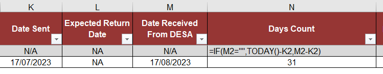
I am trying to get a cell to populate a cell with NA instead of #VALUE! At the moment I am using the error conformational format to hide the #VALUE! By white background abd white font the formula I'm using is =IF(M2="",TODAY()-K2,M2-K2)

 

[Fluff]

How about

=iferror(IF(M2="",TODAY()-K2,M2-K2),"NA")

 

[Georgiboy]

You can also swap the "NA" for NA() if you want to return an actual #N/A error.

 

[Tryingtoresolve]

Thank you that works great

 

[Fluff]

Glad we could help & thanks for the feedback.

 

[Tryingtoresolve]

I'm now struggling with a conditional format to work I'm trying to get one cell to change colour if higher than another I can make this work but I'm trying to get it to ignore N/A within the column I've tried using this =IF(O2>U2),"N/A) it accepts it and changes the cell where its higher but still highlights N/A

 

[Fluff]

As this is a totally different question, it needs a new thread. Thanks

 

[Tryingtoresolve]

As this is a totally different question, it needs a new thread. Thanks

OK thank you