How to make a Data Validation Dependent Drop Down List From the precedent Row?

[Lacan]

Hello Guys,

Have this massive extent List that would like to make a Data Validation Dependent Drop Down List from the precedent row.

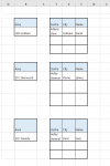
Will give you a sample data with 4 examples to be very clear that what is the goal in order to choose from Data Validation Dependent Drop Down List from the precedent row.

Can you help me?

Thanks a lot.

Book1
	B	C	D	E	F	G	H	I	J	K
2	Brick	Center	City	Name			Brick	Center	City	Name
3	299 Lx - Amadora (MÁgua - Sul)	CENTRO CLINICO AVENIDA	Amadora	Anna		Example 1	299 Lx - Amadora (MÁgua - Sul)	CENTRO CLINICO AVENIDA	Amadora	Anna
4	299 Lx - Amadora (MÁgua - Sul)	CENTRO CLINICO AVENIDA	Amadora	Anna Simon		Example 2	300 Lx - Amadora (MÁgua - Sul)	Clínica LAR MEDICO	Samouco	Anna
5	299 Lx - Amadora (MÁgua - Sul)	CENTRO CLINICO AVENIDA	Amadora	Aladin		Example 3	301 Lx - Amadora (MÁgua - Sul)	Clínica LAR JONH	Amadora	Luzia
6	299 Lx - Amadora (MÁgua - Sul)	CENTRO CLINICO AVENIDA	Amadora	Serge		Example 4	302 Lx - Amadora (MÁgua - Sul)	Clínica MEDICA SA	Lisboa	Pedro
7	299 Lx - Amadora (MÁgua - Sul)	CENTRO CLINICO AVENIDA	Amadora	Fernando
8	299 Lx - Amadora (MÁgua - Sul)	CENTRO CLINICO AVENIDA	Amadora	Blyde
9	299 Lx - Amadora (MÁgua - Sul)	CENTRO CLINICO AVENIDA	Amadora	Dynom
10	300 Lx - Amadora (MÁgua - Sul)	CENTRO CLINICO AVENIDA	Amadora	Venom
11	300 Lx - Amadora (MÁgua - Sul)	CENTRO CLINICO FRANK	Amadora	Yalan
12	300 Lx - Amadora (MÁgua - Sul)	Clínica LAR MEDICO	Samouco	Anna
13	300 Lx - Amadora (MÁgua - Sul)	Clínica LAR MEDICO	Samouco	Costa
14	300 Lx - Amadora (MÁgua - Sul)	Clínica LAR MEDICO	Samouco	Maria
15	300 Lx - Amadora (MÁgua - Sul)	Clínica LAR MEDICO	Samouco	Cesar
16	300 Lx - Amadora (MÁgua - Sul)	Clínica LAR MEDICO	Samouco	Carlos
17	301 Lx - Amadora (MÁgua - Sul)	Hospital	Amadora	Maria
18	301 Lx - Amadora (MÁgua - Sul)	Clínica LAR JONH	Amadora	Jesus
19	301 Lx - Amadora (MÁgua - Sul)	Clínica LAR JONH	Amadora	Maria
20	301 Lx - Amadora (MÁgua - Sul)	Clínica LAR JONH	Amadora	Luzia
21	301 Lx - Amadora (MÁgua - Sul)	Clínica MEDICA SA	Lisboa	Guilherme
22	302 Lx - Amadora (MÁgua - Sul)	Clínica MEDICA SA	Lisboa	Rogerio
23	302 Lx - Amadora (MÁgua - Sul)	Clínica MEDICA SA	Lisboa	Pedro
24	302 Lx - Amadora (MÁgua - Sul)	Dr Peter Sa	Samouco	Albino
25	302 Lx - Amadora (MÁgua - Sul)	Consultorio Dr King	Lisboa	Fernando
Folha6

 

[Lacan]

Hi, Lacan
If you already have Dynamic Array function in your Office 365, then you can try this example of dependent data validation (but it's only 3 column data validation). It uses VBA + formula.
Let me know if you're interested in this method & need help to apply it for 4 column data validation in your workbook.
dhee - 3 data validation, dependent, dynamic array 365.xlsm

'=================================================================================================
'=============== YOU MAY NEED TO ADJUST THE CODE IN THIS PART: ===================================

'sheet's name where the list for data validation is located. [in the sample: sheet "sheet2"]
Private Const sList As String = "sheet2"

'table's name where the list for data validation is located. [in the sample: "Table1"]
Private Const sTable As String = "Table1"

'the helper column
Private Const xH As String = "E"

'range where data validation is located
Private Const sDV1 As String = "B2:B10"  ' for data validation 1
Private Const sDV2 As String = "C2:C10"  ' for data validation 2
Private Const sDV3 As String = "D2:D10"  ' for data validation 2

'==================================================================================================
'==================================================================================================

Private Sub Worksheet_SelectionChange(ByVal Target As Range)

If Target.Cells.CountLarge > 1 Then Exit Sub
'    On Error GoTo skip:
    If Not Intersect(Target, Union(Range(sDV1), Range(sDV2), Range(sDV3))) Is Nothing Then
        Dim f As Range
        Dim MN As String, tx1 As String, tx2 As String, tx3 As String
       
        Application.EnableEvents = False
        Sheets(sList).Columns(xH).ClearContents

        Set f = Sheets(sList).ListObjects(sTable).DataBodyRange
        tx1 = f.Columns(1).Address
        tx2 = f.Columns(2).Address
        tx3 = f.Columns(3).Address
        MN = Me.Name & "!"
       
        With Sheets(sList).Range(xH & 1)
            If Target.Column = Range(sDV1).Column Then
                .Value = "=UNIQUE(" & tx1 & ")"
                           
            ElseIf Target.Column = Range(sDV2).Column And Target.Offset(, -1) <> "" Then
                .Value = "=UNIQUE(FILTER(" & tx2 & "," & tx1 & "=" & MN & Target.Offset(, -1).Address & "))"
           
            ElseIf Target.Column = Range(sDV3).Column And Target.Offset(, -1) <> "" And Target.Offset(, -2) <> "" Then
                .Value = "=UNIQUE(FILTER(" & tx3 & ",(" & tx1 & "=" & _
                MN & Target.Offset(, -2).Address & ")*(" & tx2 & "=" & MN & Target.Offset(, -1).Address & ")))"

            End If
        End With
       
        Application.EnableEvents = True

    End If


End Sub


Private Sub Worksheet_Change(ByVal Target As Range)
If Target.Cells.CountLarge <> 1 Then Exit Sub
    If Not Intersect(Target, Union(Range(sDV1), Range(sDV2))) Is Nothing Then
       
        Application.EnableEvents = False
            If Target.Column = Range(sDV1).Column Then
            Target.Offset(, 1).Resize(, 2).ClearContents
            ElseIf Target.Column = Range(sDV2).Column Then
            Target.Offset(, 1).ClearContents
            End If
        Application.EnableEvents = True
   
    End If
End Sub

Thank you ver much my Friend.

However to make crystal clear the goals I make another post thread with all data that everyone understands what want to achieve.

So please give your opinnion:

How to create a Data Validation Drop-down list based on another Data Validation Drop-down list in precedent Row? (Cascade Drop Down Menu)

Thanks again.

 

[Akuini]

So please give your opinnion:

Sorry, I don't know how to do that without VBA.

 

[Toadstool]

I see the duplicated thread has been closed so I'll repost here my very slow (5 seconds per cycle on my laptop) response using Excel 2016 with CELL ADDRESS and INDIRECT functions.

Lacan.xlsx
	A	B	C	D	E	F	G	H	I	J	K	L	M	N	O
1												$L$4:$L$6	$M$4:$M$5	$N$4:$N$5	$O$4:$O$5
2		Area	Centre	City	Name		Area	Centre	City	Name			$G$5	$H$5	$I$5
3		299 Gotham	Adams Clinic	Gotham	John		302 Xanadu	Holby General	Gotham	Michael		Area	Centre	City	Name
4		299 Gotham	Adams Clinic	Gotham	Sarah		301 Sherwood	Faith Medical	Rome	Gillian		299 Gotham	Adams Clinic	Gotham	Margaret
5		299 Gotham	Adams Clinic	Gotham	Simon		299 Gotham	Adams Clinic	Paris	James		301 Sherwood	Faith Medical	Paris	James
6		299 Gotham	Adams Clinic	Paris	Margaret							302 Xanadu
7		299 Gotham	Adams Clinic	Paris	James
8		299 Gotham	Faith Medical	Paris	Peter
9		299 Gotham	Faith Medical	Gotham	Vanessa
10		301 Sherwood	Faith Medical	Gotham	Susan
11		301 Sherwood	Faith Medical	Rome	Gillian
12		301 Sherwood	Holby General	Rome	Alex
13		301 Sherwood	Holby General	Rome	James
14		302 Xanadu	Holby General	Paris	Gary
15		302 Xanadu	Holby General	Gotham	Michael
16		302 Xanadu	Clinic Osso	Paris	Thomas
17		302 Xanadu	Clinic Osso	Milan	Thomas
18
Sheet1

Cell Formulas
Range	Formula
L1:O1	L1	=CELL("address",L4)&":"&ADDRESS(COUNTIF(L$4:L$1000,"> ")+ROW(L$3),COLUMN())
M2:O2	M2	=ADDRESS(COUNTIF(G$3:G$10,"> ")+ROW(G$2),COLUMN(G$2))
L4:L18	L4	=INDEX(B$3:B$2500,MATCH(0,INDEX(COUNTIF(L$3:L3,B$3:B$2500),),0))&""
M4:M18	M4	=IFERROR(INDEX(C$3:C$2500,AGGREGATE(15,6,ROW(C$3:C$2500)-ROW($C$2)/((B$3:B$2500=INDIRECT(M$2))*(COUNTIF(M$3:M3,C$3:C$2500)=0)),1)),"")
N4:N18	N4	=IFERROR(INDEX(D$3:D$2500,AGGREGATE(15,6,ROW(D$3:D$2500)-ROW($C$2)/((C$3:C$2500=INDIRECT(N$2))*(B$3:B$2500=INDIRECT(M$2))*(COUNTIF(N$3:N3,D$3:D$2500)=0)),1)),"")
O4:O18	O4	=IFERROR(INDEX(E$3:E$2500,AGGREGATE(15,6,ROW(E$3:E$2500)-ROW($C$2)/((D$3:D$2500=INDIRECT(O$2))*(C$3:C$2500=INDIRECT(N$2))*(B$3:B$2500=INDIRECT(M$2))*(COUNTIF(O$3:O3,E$3:E$2500)=0)),1)),"")

Cells with Data Validation
Cell	Allow	Criteria
G3:J12	List	=INDIRECT(L$1)

 

[Lacan]

Dear Toadstool,

U are the man, thanks again pal.

However want make a last small change in the structure like this:

1. Want to make tables with validation drop menu each one correletad with the corresponding reference in the R column.

2. The reference cell in the R column its any value in data validation menu.

ALL DATA:

Book1
	B	C	D	E	F	G	H	I	J	K	L	M	N	O	P	Q	R	S	T	U	V	W
1											$L$4:$L$6	$M$4:$M$5	$N$4:$N$5	$O$4:$O$6
2	area	Centre	City	Name		Area	Centre	City	Name			$G$4	$H$3	$I$3
3	299 Gotham	Adams Clinic	Gotham	John		299 Gotham	Adams Clinic	Gotham	John		Area	Centre	City	Name			299 Gotham		Centre	City	Name
4	299 Gotham	Adams Clinic	Gotham	Sarah		299 Gotham					299 Gotham	Adams Clinic	Gotham	John					Adams Clinic	Gotham	Sarah
5	299 Gotham	Adams Clinic	Gotham	Simon							301 Sherwood	Faith Medical	Paris	Sarah
6	299 Gotham	Adams Clinic	Paris	Margaret							302 Xanadu			Simon
7	299 Gotham	Adams Clinic	Paris	James
8	299 Gotham	Faith Medical	Paris	Peter													301 Sherwood		Centre	City	Name
9	299 Gotham	Faith Medical	Gotham	Vanessa															Holby General	Rome	James
10	301 Sherwood	Faith Medical	Gotham	Susan
11	301 Sherwood	Holby General	Rome	Gillian
12	301 Sherwood	Holby General	Rome	Alex
13	301 Sherwood	Holby General	Rome	James													302 Xanadu		Centre	City	Name
14	302 Xanadu	Holby General	Paris	Gary															Holby General	Paris	Gary
15	302 Xanadu	Holby General	Gotham	Michael
16	302 Xanadu	Clinic Osso	Paris	Thomas
17	302 Xanadu	Clinic Osso	Milan	Thomas
Folha4

Cell Formulas
Range	Formula
L1, M1:O1	L1	=CELL("endereço",L4)&":"&ADDRESS(COUNTIF(L$4:L$1000,"> ")+ROW(L$3),COLUMN())
M2:O2	M2	=ADDRESS(COUNTIF(G$3:G$10,"> ")+ROW(G$2),COLUMN(G$2))
L4:L15	L4	=INDEX(B$3:B$2500,MATCH(0,INDEX(COUNTIF(L$3:L3,B$3:B$2500),),0))&""
M4:M15	M4	=IFERROR(INDEX(C$3:C$2500,AGGREGATE(15,6,ROW(C$3:C$2500)-ROW($C$2)/((B$3:B$2500=INDIRECT(M$2))*(COUNTIF(M$3:M3,C$3:C$2500)=0)),1)),"")
N4:N15	N4	=IFERROR(INDEX(D$3:D$2500,AGGREGATE(15,6,ROW(D$3:D$2500)-ROW($C$2)/((C$3:C$2500=INDIRECT(N$2))*(B$3:B$2500=INDIRECT(M$2))*(COUNTIF(N$3:N3,D$3:D$2500)=0)),1)),"")
O4:O15	O4	=IFERROR(INDEX(E$3:E$2500,AGGREGATE(15,6,ROW(E$3:E$2500)-ROW($C$2)/((D$3:D$2500=INDIRECT(O$2))*(C$3:C$2500=INDIRECT(N$2))*(B$3:B$2500=INDIRECT(M$2))*(COUNTIF(O$3:O3,E$3:E$2500)=0)),1)),"")

Named Ranges
Name	Refers To	Cells
_FilterDatabase	=Folha4!$B$2:$E$17	L4:O15
area	=Folha4!$B$3:$B$17	L4:O15
Centre	=Folha4!$C$3:$C$17	M4:O15
City	=Folha4!$D$3:$D$17	N4:O15
Name	=Folha4!$E$3:$E$17	O4:O15

Cells with Conditional Formatting
Cell	Condition		Cell Format	Stop If True
B3:E17	Expression	=contar.ses($B$3:$B$17;$G1048570;$C$3:$C$17;$H1048570)	text	NO

Cells with Data Validation
Cell	Allow	Criteria
G3:J12	List	=INDIRETO(L$1)
T9:V11	List	=INDIRETO(Y$1)
T4:V6	List	=INDIRETO(Y$1)
T14:V16	List	=INDIRETO(Y$1)

Can you help with the formulas?

Again Toadstool, dont have words to express my gratitude.

 

[Toadstool]

Hi Lacan,

I'm not sure I understand the change. Are you saying you want to replace the input area format in columns G, H, I and J (all dropdown Data Validation lists) with a similar approach but using the format in columns R, S, T, U and V?

So column R would have a Data Validation list offering each unique Area, then the three rows for T, U and V would offer Centre, City and Name only under that Area?

At the moment I use the number of Areas entered to figure out which row is being populated but with the new style that probably would not work well. I guess I could use =CELL("Address") to see what was the last active cell, e.g. if it was R3 then column M would know to offer Centre from the R3 content, but that will take a while to figure out.

 

[Lacan]

Hi Toadstool,

To resume and to clarify even better:

1. Yes, want a similar approach - dropdown Data Validation lists only in this tables range T4:V6 ; T9:V11 and T14:V16 offering Centre, City and Name only under that Area (in column R).

2. Acording with data refence in column R (Area) should get the corresponding Centre, City and Name in this tables.

Examples:

R3 (Area) should only corresp Centre, City and Name in table range T4:V6;
R8 (Area) should only corresp Centre, City and Name in table T9:V11;
R13 (Area) should only corresp Centre, City and Name in table T14:V16;

3. Ask for not worry with data validation menu - unique values in column R.

Thanks again Pal.

 

[Toadstool]

Lacan,

Even slower to support this format. Each section must be completed left to right as it build the completed Data Validation list from the entries just made..

Lacan3.xlsx
	B	C	D	E	F	G	H	I	J	K	L	M	N	O	P	Q	R
1												$M$4:$M$6	$N$4:$N$5	$O$4:$O$5	$P$4:$P$5	Active	Address
2	Area	Centre	City	Name		Area		Centre	City	Name			$G$3	$I$5	$J$5	$K$5	$G$3
3	299 Gotham	Adams Clinic	Gotham	John		299 Gotham		Adams Clinic	Gotham	Sarah		Area	Centre	City	Name
4	299 Gotham	Adams Clinic	Gotham	Sarah				Faith Medical	Paris	Peter		299 Gotham	Adams Clinic	Gotham	Margaret
5	299 Gotham	Adams Clinic	Gotham	Simon				Adams Clinic	Paris	Margaret		301 Sherwood	Faith Medical	Paris	James
6	299 Gotham	Adams Clinic	Paris	Margaret								302 Xanadu
7	299 Gotham	Adams Clinic	Paris	James		Area		Centre	City	Name
8	299 Gotham	Faith Medical	Paris	Peter		301 Sherwood		Holby General	Rome	James
9	299 Gotham	Faith Medical	Gotham	Vanessa				Faith Medical	Rome	Gillian
10	301 Sherwood	Faith Medical	Gotham	Susan
11	301 Sherwood	Faith Medical	Rome	Gillian
12	301 Sherwood	Holby General	Rome	Alex		Area		Centre	City	Name
13	301 Sherwood	Holby General	Rome	James		302 Xanadu		Faith Medical
14	302 Xanadu	Holby General	Paris	Gary
15	302 Xanadu	Holby General	Gotham	Michael
Sheet1

Cell Formulas
Range	Formula
M1:P1	M1	=CELL($R$1,M4)&":"&ADDRESS(COUNTIF(M$4:M$1000,"> ")+ROW(M$3),COLUMN())
N2	N2	=R2
O2:P2	O2	=ADDRESS(ROW(INDIRECT($Q$2)),COLUMN(I$1))
Q2	Q2	=CELL($R$1)
R2	R2	=CHOOSE(MIN(INT(ROW(INDIRECT($Q$2))+4)/5,3),CELL($R$1,G3),CELL(R1,G8),CELL($R$1,G13))
M4:M15	M4	=INDEX(B$3:B$2500,MATCH(0,INDEX(COUNTIF(M$3:M3,B$3:B$2500),),0))&""
N4:N15	N4	=IFERROR(INDEX(C$3:C$2500,AGGREGATE(15,6,ROW(C$3:C$2500)-ROW($C$2)/((B$3:B$2500=INDIRECT(N$2))*(COUNTIF(N$3:N3,C$3:C$2500)=0)),1)),"")
O4:O15	O4	=IFERROR(INDEX(D$3:D$2500,AGGREGATE(15,6,ROW(D$3:D$2500)-ROW($C$2)/((C$3:C$2500=INDIRECT(O$2))*(B$3:B$2500=INDIRECT(N$2))*(COUNTIF(O$3:O3,D$3:D$2500)=0)),1)),"")
P4:P15	P4	=IFERROR(INDEX(E$3:E$2500,AGGREGATE(15,6,ROW(E$3:E$2500)-ROW($C$2)/((D$3:D$2500=INDIRECT(P$2))*(C$3:C$2500=INDIRECT(O$2))*(B$3:B$2500=INDIRECT(N$2))*(COUNTIF(P$3:P3,E$3:E$2500)=0)),1)),"")

Cells with Data Validation
Cell	Allow	Criteria
G3,G8,G13	List	=INDIRECT($M$1)
R1	List	endereço,Address
I3:I5,I8:I10,I13:I15	List	=INDIRECT($N$1)
J3:J5,J8:J10,J13:J15	List	=INDIRECT($O$1)
K3:K5,K8:K10,K13:K15	List	=INDIRECT($P$1)

 

[Lacan]

Dear Toadstool,

First thank you very much - helped a lot.

Im now making the first tests - so far so great.

Last question - want to add another Area, Centre, City Name in G17 cell order.

In that case what which formulas do I have to to update and how so they can work all together?

Thanks again my friend.

 

[Toadstool]

Select G12 to K15, copy then paste to G17.

 

[Lacan]

Dear Toadstool,

Just copy to another sheet but doesnt work.

What Im doing wrong?

Thanks again pal.