How to return value of first non blank cell for each different account number?

[Kelvinator1]

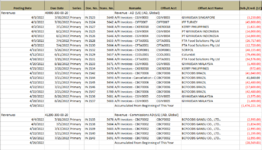
I am trying to pull in the value of a certain account number that is 7 columns to the right of the account number, and then go down to the first non-blank cell in that column. Then I want to repeat for the next account number and so on. So, in the example, for account number 40000-300-00-20, I am trying to get the value of (1,474,221.16), which is also on the same line as "Accumulated From Beginning of This Year." Then I want to go to the next account number, 41200-300-00-20 and get the value (28,569.05). These are both the values in the last non-blank cells in Column I for each respective account number. These amounts will be pulled into another sheet as part of the P&L. What is the easiest way to do this? Any help would be greatly appreciated!

 

[jolivanes]

Do you get any result from running this?

Sub Maybe()
Dim c As Range, r As Long
    For Each c In Range("A1:A" & Cells(Rows.Count, 1).End(xlUp).Row)
        If c.Value = "Revenues" Then 
            r = c.Row 
            MsgBox Cells(r + 1, 9).End(xlDown).Value
        End If
    Next c
End Sub

Upload a representative copy of your file to a free cloud storage like dropbox and let us know the password for it so we can have a look.

 

[Eric W]

Maybe something like this:

Book1 (version 1).xlsb
	A	B	C	D	E	F	G	H	I	J	K	L	M
1	Posting Date	Due Date	Series	Doc. No.	Trans. No	Remarks	Offset Acct	Offset Acct Name	Deb./Cred.(LC)			Account	Amount
2	Revenues	40000-300-00-20										40000-300-00-20	$ (500.00)
3		1							$ 1.00			41200-300-00-20	$ (750.00)
4		2							$ 1.00
5		3							$ 1.00
6		4							$ 1.00
7		5				Accumulated from Beginning of This Year			$ (500.00)
8
9	Revenues	41200-300-00-20							$ 2.00
10		6							$ 2.00
11		7							$ 2.00
12		8				Accumulated from Beginning of This Year			$ (750.00)
13
Sheet12

Cell Formulas
Range	Formula
L2:M3	L2	=LET(w,FILTER(B2:I100,(A2:A100="Revenues")+(LEFT(F2:F100,5)="Accum")),s,SEQUENCE(ROWS(w)/2,,,2),CHOOSE({1,2},INDEX(w,s,1),INDEX(w,s+1,8)))
Dynamic array formulas.

This is based on the account always being in the line that says Revenues, and the amount always in the next line that has Accumulated in it.

 

[jolivanes]

The so called empty cells are probably not empty as such.

Eric made me think to attack it differently.
Change references where required.

Sub Maybe_3()
Dim c As Range
    For Each c In Range("F1:F" & Cells(Rows.Count, 6).End(xlUp).Row)
        If InStr(c, "Accumulated") <> 0 Then Sheets("Sheet2").Cells(Sheets("Sheet2").Rows.Count, 1).End(xlUp).Offset(1).Value = c.Offset(, 3).Value
    Next c
End Sub

 

[Shortmeister1]

If you've got no option but to use the data dump, then I would do it in Power Query and ditch the VBA. PQ is specifically designed for data cleansing and is without a doubt, the biggest gamechanger in Excel in over 20 years.

1. Load your data into Power Query from the data tab on the ribbon.
2. Create a new conditional column eg. IF Posting Date = Revenues then new conditional column = Due Date else Null
3. Fill Down your new column.
4. Now filter out every record that has Posting Date = Revenues, Posting Date = "" and Due Date = "".
5. Close and Load the dataset to a new worksheet and watch the magic happen....

5 easy steps that can be rerun just by right clicking and refreshing your table!

 

[Eric W]

Shorter version of my formula:

=CHOOSE({1,2},FILTER(B2:B100,A2:A100="Revenues"),FILTER(I2:I100,LEFT(F2:F100,5)="Accum"))

 

[Kelvinator1]

Sub Maybe()
Dim c As Range
For Each c In Range("A1:A" & Cells(Rows.Count, 1).End(xlUp).Row)
If c.Value = "Revenues" Then Sheets("Month IS Detailed").Cells(Sheets("Month IS Detailed").Rows.Count, 1).End(xlUp).Offset(1).Value = c.Offset(1, 8).End(xlDown).Value
Next c
End Sub

I have no idea what I am doing here. I just copied and pasted your code into a new macro that I created, then selected Run. Nothing happens. I don't know how else to do it.

 

[jolivanes]

What about the code from Post #13 or Eric's solution?
I suspect that the empty looking cells have non printable characters.

 

[Kelvinator1]

Jolivanes:

I don't know what I'm doing. I copied the text, changed the sheet name, then pasted it into a macro:

Sub Maybe_3()
Dim c As Range
For Each c In Range("F1:F" & Cells(Rows.Count, 6).End(xlUp).Row)
If InStr(c, "Accumulated") <> 0 Then Sheets("YTD IS Detailed").Cells(Sheets("YTD IS Detailed").Rows.Count, 1).End(xlUp).Offset(1).Value = c.Offset(, 3).Value
Next c
End Sub

Then I go to Macros>View Macros, select Maybe _3, then click Run. Absolutely nothing happens. What is it supposed to be doing? Am I doing this all wrong?

 

[Kelvinator1]

If you've got no option but to use the data dump, then I would do it in Power Query and ditch the VBA. PQ is specifically designed for data cleansing and is without a doubt, the biggest gamechanger in Excel in over 20 years.

1. Load your data into Power Query from the data tab on the ribbon.
2. Create a new conditional column eg. IF Posting Date = Revenues then new conditional column = Due Date else Null
3. Fill Down your new column.
4. Now filter out every record that has Posting Date = Revenues, Posting Date = "" and Due Date = "".
5. Close and Load the dataset to a new worksheet and watch the magic happen....

5 easy steps that can be rerun just by right clicking and refreshing your table!

Martinshort, this may be the way to go but I've never used Power Query before and your instructions weren't completely clear, so I couldn't get it to work properly. Just so you know, not every category in the Posting Date column says "Revenues." As the report goes down, the categories change, like "Cost of Sales," "Other Revenues and Expenses," etc. I have no idea why SAP puts the categories into the same column as the Posting Date. I'm still not sure what this extra column is supposed to do, as when I followed your instructions, everything in that column says "Null." I know I'm doing something wrong, but I'm not even sure how this is supposed to extract the balance in the Deb/Cred column, which is the number I am trying to pull for each different account (that is buried in the Due Date column).

 

[jolivanes]

Everything I suggested worked on a mock-up so I really don't know what to say.