If 2 columns contain text from 2 ranges, insert text

[chestnutgreen]

Hello This is my first post. I've been a longtime lurker and always found what I needed without posting. But this time I've searched for a long time and tried different formulas without success.


I am trying to construct a formula that will return certain text based on the text in two columns. Each column is to be matched with a different named range.

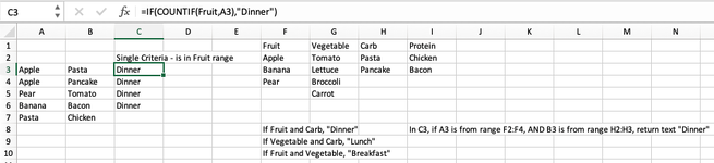
For example: A3 contains "apple" and B3 contains "pasta". I want a formula for C3 that determines if A3 is from range F2:F4 (a list of fruit), and B3 is from range H2:H3 (a list of carbs), return text "Dinner".

Separately I would specify if the A value is from the carb range and the B value is from the protein language, the returned C text is "Lunch".

I would do this for about six conditions (eg Breakfast, Lunch, Snack, Dinner, Dessert, Midnight). Each range might have 20+ items.


I can do a simple evaluation based on one column but I have been frustrated trying to get one cell to evaluate two columns.
This works for one column:

=IF(COUNTIF(Fruit,A3),"Dinner","")

Screenshot attached - I can't get the mini-sheet to work with my older version of Excel.

Any help would be most appreciated.

 

[SunnyAlv]

Like This ?

=LET(
FA,COUNTIF($F$2:$F$4,A3),
VA,COUNTIF($G$2:$G$5,A3),
CA,COUNTIF($H$2:$H$3,A3),
PA,COUNTIF($I$2:$I$3,A3),
FB,COUNTIF($F$2:$F$4,B3),
VB,COUNTIF($G$2:$G$5,B3),
CB,COUNTIF($H$2:$H$3,B3),
PB,COUNTIF($I$2:$I$3,B3),
IF(FA+CB>=2,"Dinner",IF(VA+CB>=2,"Lunch","Breakfast")))

Copy my Formula to Column C3, and u can add some Criteria ya

 

[Peter_SSs]

@SunnyAlv
The OP's profile shows excel 2016 so they would not have the LET function.

@chestnutgreen
Welcome to the MrExcel board!

Could you use something like this?
I have assumed that any particular food item would appear in only one of the categories in columns F:I

23 09 14.xlsm
	A	B	C	D	E	F	G	H	I	J	K	L
1						Fruit	Vegetable	Carb	Protein		Combo	Meal
2						Apple	Tomato	Pasta	Chicken		Fruit|Carb|Fruit	Dinner
3	Apple	Pasta	Dinner			Banana	Lettuce	Pancake	Bacon		Vegetable|Carb|Vegetable	Lunch
4	Apple	Pancake	Dinner			Pear	Broccoli				Fruit|Vegetable|Fruit	Breakfast
5	Pear	Tomato	Breakfast				Carrot
6	Banana	Bacon	??
7	Pasta	Chicken	??
8	Pancake	Carrot	Lunch
Meals

Cell Formulas
Range	Formula
C3:C8	C3	=IFNA(INDEX(L$2:L$4,MATCH("*"&INDEX(F$1:I$1,SUMPRODUCT((F$2:I$100=A3)*(COLUMN(F$2:I$2)-COLUMN(F$2)+1)))&"|"&INDEX(F$1:I$1,SUMPRODUCT((F$2:I$100=B3)*(COLUMN(F$2:I$2)-COLUMN(F$2)+1)))&"*",K$2:K$4,0)),"??")

 

[chestnutgreen]

@SunnyAlv
Thank you - LET would be good to try. I might just finally have to get around to updating to 365. Hope Microsoft has you on commission

@Peter_SSs
Brilliant - it works and I've been able to adapt it, although I'm still learning all the parameters. Thank you for going to such detail to make this work - much appreciated.
To answer your question, yes - each item will appear only once in the index.

When there are items in column A *and* B that do not appear at all in the index, the formula gives me #VALUE! How can I adopt the formula so it gives no return or error?
When there is an item in column A *or* B that does not appear in the index, in the formula I've replaced "??" with "" and that has worked.

Thank you again to you both.

 

[Peter_SSs]

Would something like this be suitable then?

23 09 14.xlsm
	A	B	C	D	E	F	G	H	I	J	K	L
1						Fruit	Vegetable	Carb	Protein		Combo	Meal
2						Apple	Tomato	Pasta	Chicken		Fruit|Carb|Fruit	Dinner
3	Apple	Pasta	Dinner			Banana	Lettuce	Pancake	Bacon		Vegetable|Carb|Vegetable	Lunch
4	Apple	Pancake	Dinner			Pear	Broccoli				Fruit|Vegetable|Fruit	Breakfast
5	Pear	Tomato	Breakfast				Carrot				x|y
6	Salt	Pepper
7	Salt	Pasta
8	Pasta	Salt
9	Pasta	Chicken
10	Pancake	Carrot	Lunch
Meals (2)

Cell Formulas
Range	Formula
L5	L5	=""
C3:C10	C3	=IFNA(INDEX(L$2:L$5,MATCH("*"&IF(COUNTIF(F$2:I$100,A3)=1,INDEX(F$1:I$1,SUMPRODUCT((F$2:I$100=A3)*(COLUMN(F$2:I$2)-COLUMN(F$2)+1))),"x")&"|"&IF(COUNTIF(F$2:I$100,B3)=1,INDEX(F$1:I$1,SUMPRODUCT((F$2:I$100=B3)*(COLUMN(F$2:I$2)-COLUMN(F$2)+1))),"y")&"*",K$2:K$5,0)),"")