IF Formula with Exception

[Dandelion3]

Hi everyone.

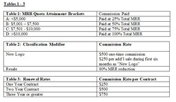
I have an IF formula in place for a file that i'm working on. Final value is based on a percentage, but there is one person whose final value should be based on a dollar value instead. The current formula conditions apply no matter what the user name is, but there is one person who is an exception, so I need to make adjustments to basically say "All else applies, but for this particular user, it should be something different" while keeping everything else in place. I still want everything on the same tab. Hopefully that makes sense. Do i just add a comma & put that IF statement on the end? Will that change everything else?

 

[Dandelion3]

Does column R only come into play with John Doe or all other owners too? And what does column R do? Is it a multiplier? Or some other code to determine $ amount?

Column R is for all owners. Column R divided by 12 gives the value for Column U. The formula bar shown is for Column V. It's saying for a 1 year contract, the accelerator should be 0, for a 2 year contract, the accelerator should be 15% of the base commission (Column S), for a 3 year contract, it should be 35%, and for 4 or more years, it should be 50% of the base commission......... But for John Doe, that accelerator base does not apply. For John Doe the conditions(that I want to ADD to the current formula) are below: *using dummy numbers*

1.If the OPP MRR (Column N) is <$5,000 commission should be paid at 2% of column N.... $5,001 - $7,500 should be paid at 5%..... $7,5001-$10,000 should be paid at 8%, >$10,000 paid at 10%
2. If "New Logo" , $30
3. If 1 year contract (contract term reflected in column U based off column R), $20 ... If 2 year contract $30..... If 3 years or greater, $50
***Column Z "CLASSIFICATON MODIFIER** is where this dollar amount contingent upon these conditions should be reflected.

1 + 2 + 3 = Total commission pay

Formula Bar is for column AA

 

[dreid1011]

Column R is for all owners. Column R divided by 12 gives the value for Column U. The formula bar shown is for Column V. It's saying for a 1 year contract, the accelerator should be 0, for a 2 year contract, the accelerator should be 15% of the base commission (Column S), for a 3 year contract, it should be 35%, and for 4 or more years, it should be 50% of the base commission......... But for John Doe, that accelerator base does not apply. For John Doe the conditions(that I want to ADD to the current formula) are below: *using dummy numbers*

1.If the OPP MRR (Column N) is <$5,000 commission should be paid at 2% of column N.... $5,001 - $7,500 should be paid at 5%..... $7,5001-$10,000 should be paid at 8%, >$10,000 paid at 10%
2. If "New Logo" , $30
3. If 1 year contract (contract term reflected in column U based off column R), $20 ... If 2 year contract $30..... If 3 years or greater, $50
***Column Z "CLASSIFICATON MODIFIER** is where this dollar amount contingent upon these conditions should be reflected.

1 + 2 + 3 = Total commission pay



View attachment 103090

Formula Bar is for column AA
View attachment 103093

Okay, but none of this seems to apply to the formula we were originally working on.

 

[Dandelion3]

Okay, but none of this seems to apply to the formula we were originally working on.

So how do I had those conditions for that one person to the formula while still having the original conditions apply to all other users, still.

 

[dreid1011]

So how do I had those conditions for that one person to the formula while still having the original conditions apply to all other users, still.

We just need to add some IFs to the formula to check for that single person. All of the conditions below need to be in column Z and added all together?

1.If the OPP MRR (Column N) is <$5,000 commission should be paid at 2% of column N.... $5,001 - $7,500 should be paid at 5%..... $7,501-$10,000 should be paid at 8%, >$10,000 paid at 10%
2. If "New Logo" , $30
3. If 1 year contract (contract term reflected in column U based off column R), $20 ... If 2 year contract $30..... If 3 years or greater, $50
***Column Z "CLASSIFICATON MODIFIER** is where this dollar amount contingent upon these conditions should be reflected.

1 + 2 + 3 = Total commission pay

 

[Dandelion3]

Ok, I'm going to try a different approach and create a separate tab for this particular person instead of trying to include it in the existing formula.

I need a formula that says: If Opp MRR (which is a dollar value in column N) is:

• <$3,000, then commission should be 25% of column N
• $3,001 - $5,500: then commission should be 50% of column N
• $5,501 - $8,000: then commission should be 75% of column N
• >$8,000: then commission should be 100% of column N

I need a 2nd formula that says:

• If B2 says "New Logo", it should be $300
• If B2 says "resale", it should be an 75% reduction of MRR (column N)

I need a 3rd formula that says, If column U (Contract years) is:

• 1, then it should be $150
• 2, then it should be $350
• 3 or greater, then it should be $650

 

[dreid1011]

Ok, I'm going to try a different approach and create a separate tab for this particular person instead of trying to include it in the existing formula.

I need a formula that says: If Opp MRR (which is a dollar value in column N) is:

• <$3,000, then commission should be 25% of column N
• $3,001 - $5,500: then commission should be 50% of column N
• $5,501 - $8,000: then commission should be 75% of column N
• >$8,000: then commission should be 100% of column N

I need a 2nd formula that says:

• If B2 says "New Logo", it should be $300
• If B2 says "resale", it should be an 75% reduction of MRR (column N)

It doesn't help that your numbers keep changing each time you state the conditions. It can be working into the existing formula, that's not the problem. I got this far earlier, does this look like what you want?

Book1
	A	B	C	D	E	F	G	H	I	J	K	L	M	N	O	P	Q	R	S	T	U	V	W	X	Y	Z	AA
1		Classification			Owner									Opp MRR	Opp aMRR	Opp NRR	COMP MRR	Initial Term	Case Commission	Renewal Commission	Contract (Years)	Accelerator Base	Accelerator Renewal	Base - Total Commission	Renewal - Total Commission	Classification Modifier	Total Commission
2		New Logo			John Doe									5050				12			1	0		50	50	302.5	30250
Sheet1

Cell Formulas
Range	Formula
U2	U2	=R2/12
V2	V2	=IF(E2<>"John Doe",IF(U2=1,0,IF(U2=2,S2*15%,IF(U2=3,S2*35%,IF(U2>=4,S2*50%,0)))),0)
Z2	Z2	=IF(E2<>"John Doe",IF(B2="Channel Driven/New Logo",80%,IF(B2="New",100%,IF(B2="New Logo",150%,IF(B2="Channel Driven",70%,IF(B2="Resale",80%,0))))),SUM(N2*LOOKUP(N2,{0,5001,7501,10001},{0.02,0.05,0.08,0.1}),IF(B2="New Logo",30,0),LOOKUP(U2,{1,2,3},{20,30,50})))
AA2	AA2	=SUM(X2:Y2)*Z2

 

[Dandelion3]

It doesn't help that your numbers keep changing each time you state the conditions. It can be working into the existing formula, that's not the problem. I got this far earlier, does this look like what you want?

Book1
	A	B	C	D	E	F	G	H	I	J	K	L	M	N	O	P	Q	R	S	T	U	V	W	X	Y	Z	AA
1		Classification			Owner									Opp MRR	Opp aMRR	Opp NRR	COMP MRR	Initial Term	Case Commission	Renewal Commission	Contract (Years)	Accelerator Base	Accelerator Renewal	Base - Total Commission	Renewal - Total Commission	Classification Modifier	Total Commission
2		New Logo			John Doe									5050				12			1	0		50	50	302.5	30250
Sheet1

Cell Formulas
Range	Formula
U2	U2	=R2/12
V2	V2	=IF(E2<>"John Doe",IF(U2=1,0,IF(U2=2,S2*15%,IF(U2=3,S2*35%,IF(U2>=4,S2*50%,0)))),0)
Z2	Z2	=IF(E2<>"John Doe",IF(B2="Channel Driven/New Logo",80%,IF(B2="New",100%,IF(B2="New Logo",150%,IF(B2="Channel Driven",70%,IF(B2="Resale",80%,0))))),SUM(N2*LOOKUP(N2,{0,5001,7501,10001},{0.02,0.05,0.08,0.1}),IF(B2="New Logo",30,0),LOOKUP(U2,{1,2,3},{20,30,50})))
AA2	AA2	=SUM(X2:Y2)*Z2

My apologies. I thought I was making it easier. Let me try what you have here. I appreciate the help so much. The numbers are changing for confidentiality purposes, so I'm throwing random numbers out and will plug the actual numbers in the spreadsheet.

 

[Dandelion3]

It doesn't help that your numbers keep changing each time you state the conditions. It can be working into the existing formula, that's not the problem. I got this far earlier, does this look like what you want?

Book1
	A	B	C	D	E	F	G	H	I	J	K	L	M	N	O	P	Q	R	S	T	U	V	W	X	Y	Z	AA
1		Classification			Owner									Opp MRR	Opp aMRR	Opp NRR	COMP MRR	Initial Term	Case Commission	Renewal Commission	Contract (Years)	Accelerator Base	Accelerator Renewal	Base - Total Commission	Renewal - Total Commission	Classification Modifier	Total Commission
2		New Logo			John Doe									5050				12			1	0		50	50	302.5	30250
Sheet1

Cell Formulas
Range	Formula
U2	U2	=R2/12
V2	V2	=IF(E2<>"John Doe",IF(U2=1,0,IF(U2=2,S2*15%,IF(U2=3,S2*35%,IF(U2>=4,S2*50%,0)))),0)
Z2	Z2	=IF(E2<>"John Doe",IF(B2="Channel Driven/New Logo",80%,IF(B2="New",100%,IF(B2="New Logo",150%,IF(B2="Channel Driven",70%,IF(B2="Resale",80%,0))))),SUM(N2*LOOKUP(N2,{0,5001,7501,10001},{0.02,0.05,0.08,0.1}),IF(B2="New Logo",30,0),LOOKUP(U2,{1,2,3},{20,30,50})))
AA2	AA2	=SUM(X2:Y2)*Z2

I entered your suggestion in column Z, and It gave me 5550%

 

[Dandelion3]

Ok, let's try to start fresh. Below is the a picture of the commission pay structure I am trying to implement for John Doe. I have also provided the current formula that applies to everyone except John Doe.

CURRENT FORMULAS:

• Column S: =IF(N2>0,N2,0)
• Column T: =Q2
• Column U: =R2/12
• Column V: =IF(U2=1,0,IF(U2=2,S2*15%,IF(U2=3,S2*35%,IF(U2>=4,S2*50%,0))))
• Column W: =IF(U2=1,0,IF(U2=2,T2*15%,IF(U2=3,T2*30%,IF(U2>=4,T2*50%,0))))
• Column X: =SUM(S2,V2)
• Column Y: =W2+T2
• Column Z: =IF(B2="Channel Driven/New Logo",80%,IF(B2="New",100%,IF(B2="New Logo",150%,IF(B2="Channel Driven",70%,IF(B2="Resale",80%,0)))))
• Column AA: =SUM(X2:Y2)*Z2

*I am open to including this structure in the current formula OR creating a new tab for John Doe only.

 

[dreid1011]

Can you provide some sample values and what you expect the result to be in AA?

I entered your suggestion in column Z, and It gave me 5550%

With the values I used, what is the result you expect?