=IF SUMPRODUCT Formula

[uk_2022]

I have got a =if sumproduct formula below

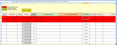
=IF(SUMPRODUCT((I9<$K$9:$K$17)*(K9>$I$9:$I$17)*(N9=$N$9:$N$17))>1,"Check","Available")

however I need the (N9=$N$9:$N$17) section to find values within the text.

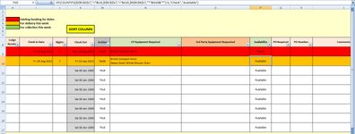
Values in column N are entered from a drop down list (a VBA allow multiple selections).

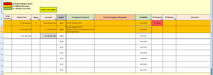
I have attached a image of my worksheet;

Example: Check in dates overlap and both rows contain "Birdie Compact Hoist" in column N, however row 10 also contains "Aquatec......." in the same cell.

Currently, column P is returning "available" as per the formula above as it is not picking up that "Birdie Compact Hoist" has appeared in both cells.

Can anyone suggest a solution how the formula can pick out matching values from the text in column N?

TIA

 

[SanjayGMusafir]

Try this -

=IF(SUMPRODUCT((I9<$K$9:$K$17)*(K9>$I$9:$I$17)*(IFERROR(FIND(N9,$N$9:$N$17),0)))>1,"Check","Available")

 

[Phuoc]

=IF(COUNTIFS($K$9:$K$17,">"&I9,$I$9:$I$17,"<"&K9,$N$9:$N$17,"*"&N9&"*")>1,"Check","Available")

 

[uk_2022]

Try this -

=IF(SUMPRODUCT((I9<$K$9:$K$17)*(K9>$I$9:$I$17)*(IFERROR(FIND(N9,$N$9:$N$17),0)))>1,"Check","Available")

Sorry this still hasn't worked, have attached image.

Dates overlap but the equipment results are different yet it still returns Check in column P

 

[uk_2022]

=IF(COUNTIFS($K$9:$K$17,">"&I9,$I$9:$I$17,"<"&K9,$N$9:$N$17,"*"&N9&"*")>1,"Check","Available")

This has worked slightly better as it returned row 10 as "available" and row 9 as "check" due to both having "Birdie......" within column N.

Ideally I need both rows to say check if they have matching values in column N.

 

[SanjayGMusafir]

Sorry this still hasn't worked, have attached image.

Dates overlap but the equipment results are different yet it still returns Check in column P

See Uploading image doesn't help in checking error.

Better upload a sample data using XL2BB utility to find what's going wrong.

 

[uk_2022]

Equipment Log Template.xlsm
	B	C	D	E	F	G	H	I	J	K		M	N	O	P	Q	R	S
8	Initals	AFA Request	Booking Ref	Booking Name	Contact Number	Contact Email	Lodge Number	Check in Date	Nights	Check Out		Archive	CP Equipment Required	3rd Party Equipment Requested	Availability	PO Required	PO Number	Comments
9								Fri 26 Aug 2022	3	Mon 29 Aug 2022		FALSE	Sunlift Micro Hoist		Check
10								Fri 26 Aug 2022	7	Fri 02 Sep 2022		FALSE	Geeco Small White Shower Chair Birdie Compact Hoist		Check
11															Check
12															Check
13															Check
14															Check
15															Check
16															Check
17															Check
Equipment

Cell Formulas
Range	Formula
K9:K17	K9	=IF(J9="","",I9+J9)
M9:M17	M9	=IF(J9="","",IF(K9<TODAY(),TRUE,FALSE))
P9:P17	P9	=IF(SUMPRODUCT((I9<$K$9:$K$17)*(K9>$I$9:$I$17)*(IFERROR(FIND(N9,$N$9:$N$17),0)))>1,"Check","Available")

Cells with Data Validation
Cell	Allow	Criteria
Q9:Q17	List	To Raise, Raised
N9:N17	List	=Lists!$A$2:$A$12
O9:O17	List	=Lists!$B$2:$B$23

 

[SanjayGMusafir]

I thing I just realized - FIND is a case sensitive while SEARCH is not you can try that -

=IF(SUMPRODUCT((I9<$K$9:$K$17)*(K9>$I$9:$I$17)*(IFERROR(SEARCH(N9,$N$9:$N$17),0)))>1,"Check","Available")

 

[uk_2022]

Sorry its still not working - it is matching overlapping dates but not matching any text in column N.

I have added overlapping dates but selected different equipment but it still returns "Check".

I only need it to return "Check" if the date overlap others AND the equipment in column N match. I.E if both rows had "Birdie Compact Hoist" within the values. (See row 10 - it also has "Geeco....." but I still need the formula to recognise that "Birdie....." appears with the text.

 

[uk_2022]

Equipment Log Template.xlsm
	B	C	D	E	F	G	H	I	J	K		M	N	O	P	Q	R	S
8	Initals	AFA Request	Booking Ref	Booking Name	Contact Number	Contact Email	Lodge Number	Check in Date	Nights	Check Out		Archive	CP Equipment Required	3rd Party Equipment Requested	Availability	PO Required	PO Number	Comments
9								Fri 26 Aug 2022	3	Mon 29 Aug 2022		FALSE	Sunlift Micro Hoist		Check
10								Fri 26 Aug 2022	7	Fri 02 Sep 2022		FALSE	Geeco Small White Shower Chair Birdie Compact Hoist		Check
11															Available
12															Available
13															Available
14															Available
15															Available
16															Available
17															Available
Equipment

Cell Formulas
Range	Formula
K9:K17	K9	=IF(J9="","",I9+J9)
M9:M17	M9	=IF(J9="","",IF(K9<TODAY(),TRUE,FALSE))
P9:P17	P9	=IF(SUMPRODUCT((I9<$K$9:$K$17)*(K9>$I$9:$I$17)*(IFERROR(SEARCH(N9,$N$9:$N$17),0)))>1,"Check","Available")

Cells with Data Validation
Cell	Allow	Criteria
Q9:Q17	List	To Raise, Raised
N9:N17	List	=Lists!$A$2:$A$12
O9:O17	List	=Lists!$B$2:$B$23