Index formula, can the column number be dynamic?

[Tirrazo]

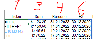
I need help to set the column number for the index formula automatically instead of static.

The formula is used in combination with LET-function and the array that this creates are returning different values.
If I would like to increase the number of columns because I want more data within the area the formula is looking, I have to manually count the columns and enter it.
I have many if the same formulas so this takes a lot of time.

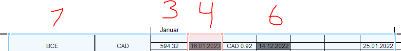
In the example I am using column 1,3,4,6 that I am getting data back from.

 

[awoohaw]

in order for the index to create a cell reference instead of value you need to preceed or follow the index portion of the function with a ":" and the cell reference that is on the other end. I don't that in your formula? can you explain in words what youre trying to do?

 

[Tirrazo]

in order for the index to create a cell reference instead of value you need to preceed or follow the index portion of the function with a ":" and the cell reference that is on the other end. I don't that in your formula? can you explain in words what youre trying to do?

Can you try to use my formula and insert it with the correct Index reference?
I am not sure how to do it

 

[awoohaw]

Please post 10-20 rows of examples comparing the worksheet results you have with what you want using xl2bb?

 

[awoohaw]

but, say you have a range of A1:Z50... and you know you want to start in cell A5 and go to the first cell that has a value of 100 in it (assume there is no 100 in cells A1:A5:
the calculation to create that range is: A5:INDEX(A1:A50,Match(100,A1:A50,0) (In this simple example you could even say Match(100,A5:A50,0) in the middle of the index statement.

 

[Tirrazo]

Testark.xlsm
	U	V	W	X	Y	Z	AA	AB	AC	AD	AE	AF	AG	AH
18
19								64.60	15.04.2021	CAD 0.10	14.03.2022			28.04.2022
20	91.20	01.03.2021	CAD 0.10	14.02.2022			02.03.2021
21
22
23
24
25
26
27
28
29
30
31
32
33
34
35
36
37	Fra dato	Til dato						Fra dato	Til dato
38	01.03.2021	31.03.2022						01.04.2021	30.04.2021
39
40	Ticker	Sum	Beregnet	EX				Ticker	Sum	Beregnet	EX
41	ENB	kr 91.20	01.03.2021	14.02.2022				BCE	kr 64.60	15.04.2021	14.03.2022
42
43
44
45
46
47
Utbk

Cell Formulas
Range	Formula
AB19	AB19	=Portf!Z22*Portf!R22
U20	U20	=Portf!X23*Portf!R23
U41:X41	U41	=LET(f,FILTER(E18:AA33,(V18:V33>=U38)*(V18:V33<=V38)),IF(ISERR(ROWS(f)),"Ingen utbytte",SORT(INDEX(f,SEQUENCE(ROWS(f)),{1,17,18,20}),4)))
AB41:AE41	AB41	=LET(f,FILTER(E18:AH33,(AC18:AC33>=AB38)*(AC18:AC33<=AC38)),IF(ISERR(ROWS(f)),"Ingen utbytte",SORT(INDEX(f,SEQUENCE(ROWS(f)),{1,24,25,27}),4)))
Dynamic array formulas.

Cells with Conditional Formatting
Cell	Condition		Cell Format	Stop If True
L18:L33,S18:S33,Z18:Z33,AG18:AG33,AN18:AN33,AU18:AU33,BB18:BB33,BI18:BI33,BP18:BP33,BW18:BW33,CD18:CD33,CK18:CK33	Cell Value	>0	text	NO

Cells with Data Validation
Cell	Allow	Criteria
AB38:AC38	List	=#REF!#
U38:V38	List	=#REF!#

So, the problem occurs if I delete the row Y or Z for example. I need help to fill in at the end under INDEX so this formula is adapting no matter how many cells are in between.

 

[Tirrazo]

but, say you have a range of A1:Z50... and you know you want to start in cell A5 and go to the first cell that has a value of 100 in it (assume there is no 100 in cells A1:A5:
the calculation to create that range is: A5:INDEX(A1:A50,Match(100,A1:A50,0) (In this simple example you could even say Match(100,A5:A50,0) in the middle of the index statement.

I am returning 4 different columns with this 1 formula and those 4 columns are specified at the very end. How can I make the INDEX return the same formulas based upon your example with Col B that only returns 1 column?

 

[awoohaw]

Your spreadsheet confuses me. It looks like your have repeating information of 6 rows and 7 columns.
If that is correct, what is it you need to do with thos 6x7 grids? When you mention formula, do you mean your big LET formula? Also, your formulas reference cells on sheet Portf, some sample frm that could help, too.

 

[Tirrazo]

Your spreadsheet confuses me. It looks like your have repeating information of 6 rows and 7 columns.
If that is correct, what is it you need to do with thos 6x7 grids? When you mention formula, do you mean your big LET formula? Also, your formulas reference cells on sheet Portf, some sample frm that could help, too.

Testark 02.02.23.xlsx
	A	B	C	D	E	F	G	H	I	J	K	L	M	N	O	P	Q	R	S	T	U	V	W	X
1	en		10	16.01.2023		14.12.2023		16	19.01.2023
2	to																22	01.03.2023		14.02.2023			02.03.2023
3
4
5	tre																23	12.03.2023		17.02.2023
6	fire									40	15.02.2023		12.01.2023	29.10.2023		16.02.2023
7	fem		11	03.01.2023		16.12.2023		17	04.01.2023
8	seks																24	18.03.2023		03.03.2023	18.03.2023		21.03.2023
9	sju																25	25.03.2023		11.03.2023
10	åtte																26	31.03.2023		21.03.2023	03.03.2023		04.04.2023
11	ni		12	13.01.2023		29.12.2023		18	16.01.2023
12	ti																27	10.03.2023		15.02.2023	27.01.2023		25.01.2023
13	elleve		13	25.01.2023		04.01.2023	12.12.2023	19	26.01.2023
14	tolv		14	13.01.2023		29.12.2023		20	16.01.2023
15	tretten																28	25.03.2023		24.02.2023			28.03.2023
16	fjorten		15	03.01.2023		13.12.2023	11.11.2023	21	04.01.2023
17	femten									50	14.02.2023		01.02.2023	25.01.2023		23.01.2023
18	seksten																29	11.03.2023		14.02.2023			14.03.2023
19	sytten
20	atten																30	22.03.2023		07.03.2023	24.02.2023		23.03.2023
21	nitten																31	11.03.2023		17.02.2023
22
23
24
25
26
27
28
29
30
31
32
33
34
35																	01.01.2023
36																	31.12.2023
37
38
39
40
41																	to	22	01.03.2023	14.02.2023
42																	seksten	29	11.03.2023	14.02.2023
43																	ti	27	10.03.2023	15.02.2023
44																	tre	23	12.03.2023	17.02.2023
45																	nitten	31	11.03.2023	17.02.2023
46																	tretten	28	25.03.2023	24.02.2023
47																	seks	24	18.03.2023	03.03.2023
48																	atten	30	22.03.2023	07.03.2023
49																	sju	25	25.03.2023	11.03.2023
50																	åtte	26	31.03.2023	21.03.2023
51
52
53
Ark1

Cell Formulas
Range	Formula
Q41:T50	Q41	=LET(f,FILTER(A1:W33,(R1:R33>=Q35)*(R1:R33<=Q36)),IF(ISERR(ROWS(f)),"Ingen utbytte",SORT(INDEX(f,SEQUENCE(ROWS(f)),{1,17,18,20}),4)))
Dynamic array formulas.

I have updated the spreadsheet now, maybe easier to see how the formula is working.

Now, for example, If I remove the column 'O', the formula changes and is not displaying what it should because the columns are hard coded in the very end of the formula.

Can you try to find a solution for not hard coding/taping in the columns at the end?