index/match 3 possible forth criteria

[KDS14589]

Hello All

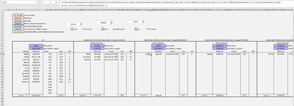
I had problem adding a fourth criteria, but with the help from a Mr Excel moderator In cell Avoid!BL18 I came up with:

=IFERROR(INDEX(statement_name,AGGREGATE(15,6,(ROW(statement_name)-ROW(Statement!$AA$10)+1)/(statement_Bal_this_month>$BM$15)/(statement_Bal_this_month<=$BM$16)/(statement_min_due>0)/(statement_name=Avoid_name_1),ROWS(Avoid!$BL$18:BL18))),"")

it's the (statement_name=Avoid_name) part.



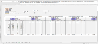
Now I've added a wrinkle by now wishing to add two more names to that criterion.



This is my last attempt:

=IFERROR(INDEX(statement_name,AGGREGATE(15,6,(ROW(statement_name)-ROW(Statement!$AA$10)+1)/(statement_Bal_this_month>$BM$15)/(statement_Bal_this_month<$BM$16)/(statement_min_due>0)/(OR(statement_name=avoid_name1,statement_name=avoid_name2,statement_name=avoid_name3)),ROWS(Avoid!$BL$18:BL18))),"")

But now it lists all the names in the list and not just the three. Hopefully this is possible, but if not or this is to involved, I'll just stick with the original.


Help would be nice.

 

[jasonb75]

You can't use the OR function as part of an array, it will return TRUE to every record in the array if any one record is actually TRUE. To create an OR array, you need to add the individual elements together then check if the result of the added elements is greater than 0 as shown below.

=IFERROR(INDEX(statement_name,AGGREGATE(15,6,(ROW(statement_name)-MIN(ROW(statement_name)+1)/(statement_Bal_this_month>$BM$15)/(statement_Bal_this_month<$BM$16)/(statement_min_due>0)/(((statement_name=avoid_name1)+(statement_name=avoid_name2)+(statement_name=avoid_name3))>0),ROWS(Avoid!$BL$18:BL18))),"")

 

[KDS14589]

You can't use the OR function as part of an array, it will return TRUE to every record in the array if any one record is actually TRUE. To create an OR array, you need to add the individual elements together then check if the result of the added elements is greater than 0 as shown below.

=IFERROR(INDEX(statement_name,AGGREGATE(15,6,(ROW(statement_name)-MIN(ROW(statement_name)+1)/(statement_Bal_this_month>$BM$15)/(statement_Bal_this_month<$BM$16)/(statement_min_due>0)/(((statement_name=avoid_name1)+(statement_name=avoid_name2)+(statement_name=avoid_name3))>0),ROWS(Avoid!$BL$18:BL18))),"")

I had to add a third ) after (statement_name=avoid_name3)) to stop the formula error but after that I still get a blank list instead of the three

 

[jasonb75]

The missing one was actually after the +1 earlier in the formula, I forgot to add the closing bracket for the MIN function. This should work correctly.

=IFERROR(INDEX(statement_name,AGGREGATE(15,6,(ROW(statement_name)-MIN(ROW(statement_name)+1))/(statement_Bal_this_month>$BM$15)/(statement_Bal_this_month<$BM$16)/(statement_min_due>0)/(((statement_name=avoid_name1)+(statement_name=avoid_name2)+(statement_name=avoid_name3))>0),ROWS(Avoid!$BL$18:BL18))),"")

 

[KDS14589]

You can't use the OR function as part of an array, it will return TRUE to every record in the array if any one record is actually TRUE. To create an OR array, you need to add the individual elements together then check if the result of the added elements is greater than 0 as shown below.

=IFERROR(INDEX(statement_name,AGGREGATE(15,6,(ROW(statement_name)-MIN(ROW(statement_name)+1)/(statement_Bal_this_month>$BM$15)/(statement_Bal_this_month<$BM$16)/(statement_min_due>0)/(((statement_name=avoid_name1)+(statement_name=avoid_name2)+(statement_name=avoid_name3))>0),ROWS(Avoid!$BL$18:BL18))),"")

I went back to your formula but for some reason I had to replace the avoid_name1w with the Excel version NOW IT WORKS
Sorry about the other reply about addding a)
THANKS FOR THE HELP

 

[jasonb75]

for some reason I had to replace the avoid_name1w with the Excel

Not exactly sure what happened there, I just used the names from the old formula. Did you see my earlier reply about the missing ) ? There was one missing, if you have added it where you mentioned then you might still get some incorrect results. The missing one was in a different part of the formula.

 

[KDS14589]

Not exactly sure what happened there, I just used the names from the old formula. Did you see my earlier reply about the missing ) ? There was one missing, if you have added it where you mentioned then you might still get some incorrect results. The missing one was in a different part of the formula.

You'er correct. The farther I went I finally would see mistakes i copied your formula and made some corrections. The avoid_name1, avoid_name2, avoid_name3 were actuallly avoid_name_1, avoid_name_2, avoid _name_3, but I'm still getting mistakes
my code i'm using is

=IFERROR(INDEX(statement_name,AGGREGATE(15,6,(ROW(statement_name)-MIN(ROW(statement_name)+1))/(statement_Bal_this_month>$BM$15)/(statement_Bal_this_month<$BM$16)/(statement_min_due>0)/(((statement_name=Avoid_name_1)+(statement_name=avoid_name_2)+(statement_name=avoid_name_3))>0),ROWS(Avoid!$BL$18:BL18))),"")

you can see from the pix I only get 2 names but the wrong ones

 

[jasonb75]

From your last reply I'm assuming that you tried to attach some additional screen captures but i don't see them in your post.

 

[KDS14589]

Sorry

 

[KDS14589]

again Sorry
I just now noticed the there pix was to large so I reworked a new one