INDEX MATCH Function Help

[jeffj13]

Hello,
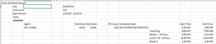
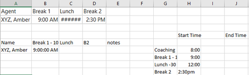
I am working with the a data set that is a schedule that shows break and lunch times. What I am trying to accomplish is listing all of the agents in column C (snippet at the bottom) and listing their Break 1, Lunch and Break 2 in column L in adjacent rows, like this:

Agent	Break 1	Lunch	Break 2
XYZ, Amber	9:00 AM	12:00 PM	2:30 PM

I am extracting the Agent name in column C with a FILTER function and ignoring blank cells into another worksheet. My attempt to extract the first break time has failed with my formula below. Any idea what I have done wrong or if this can even be done using my methodology? Thank you in advance!

 

[Coyotex3]

Perhaps you can use the Filter function to get the rest of the data as well using something like this

=FILTER(H6:H9,G6:G9=B5)

 

[Eric W]

Your original formula didn't work because the agent name and the time descriptions are not on the same line. If you know that the descriptions will always be in the same relative location (i.e. Break 1 is always 2 rows below the name), you could fix up your formula by offsetting the ranges. Here are a couple other options though:

Book1
	A	B	C	D	E
1
2
3	Name	Break 1 - 10 hour	Lunch	Break 2	Notes
4	XYZ, Amber	9:00 AM	12:00 PM	2:30 PM
5	ABC, Ed	9:15 AM	1:00 PM	2:45 PM
6	STU, Mae	11:00 AM	11:30 PM	4:30 PM
7
8
9	Name	Break 1 - 10 hour	Lunch	Break 2	Notes
10	XYZ, Amber	9:00 AM	12:00 PM	2:30 PM
11	ABC, Ed	9:15 AM	1:00 PM	2:45 PM
12	STU, Mae	11:00 AM	11:30 PM	4:30 PM
Sheet15

Cell Formulas
Range	Formula
A4:A6,A10:A12	A4	=LET(a,UNIQUE(csv!C1:C1000),FILTER(a,(a<>"")*(a<>"Agent")))
B4:D6	B4	=INDEX(csv!$L$8:$L$290,MATCH($A4,csv!$C$8:$C$292,0)+COLUMNS($A:B))
B10:D12	B10	=VLOOKUP(B$3,INDEX(csv!$K$1:$K$1000,MATCH($A10,csv!$C$1:$C$1000,0)):csv!$L$1000,2,0)
Dynamic array formulas.

The top set assumes the 3 times are always in the same relative positions. The second set searches for the agent name first, then does a VLOOKUP for the description in column K starting at the row the agent was found in. So the descriptions don't have to be in the same order, but there could be an issue if a given description is not found, since it might be found further down in the next agent's area.

Let us know if either of these might work for you.

 

[StephenCrump]

The second set searches for the agent name first, then does a VLOOKUP for the description in column K starting at the row the agent was found in. So the descriptions don't have to be in the same order, but there could be an issue if a given description is not found, since it might be found further down in the next agent's area.

That was my guess, that the data might not line up the same way.

	A	B	C	D
1
2
3	Name	Break 1 - 10 hour	Lunch	Break 2
4	XYZ, Amber	9:00 AM	12:00 PM	-
5	ABC, Ed	9:15 AM	1:00 PM	2:45 PM
6	STU, Mae	11:00 AM	11:30 PM	4:30 PM
Sheet1

Cell Formulas
Range	Formula
A4:A6	A4	=LET(a,UNIQUE(csv!C1:C1000),FILTER(a,(a<>"")*(a<>"Agent")))
B4:D6	B4	=IFERROR(VLOOKUP(B$3:D$3,IF(SCAN(,csv!$C$1:$C$1000,LAMBDA(a,b,IF(b="",a,b)))=A4,csv!K$1:L$1000),2,),"-")
Dynamic array formulas.

	A	B	C	D	E	F	G	H	I	J	K	L
1
2
3			XYZ, Amber								Break 1 - 10 hour	9:00 AM
4											Lunch	12:00 PM
5			ABC, Ed
6
7											Break 1 - 10 hour	9:15 AM
8
9											Lunch	1:00 PM
10
11											Break 2	2:45 PM
12
13
14			STU, Mae
15											Break 2	4:30 PM
16											Lunch	11:30 PM
17
18											Break 1 - 10 hour	11:00 AM
csv

 

[jeffj13]

Your original formula didn't work because the agent name and the time descriptions are not on the same line. If you know that the descriptions will always be in the same relative location (i.e. Break 1 is always 2 rows below the name), you could fix up your formula by offsetting the ranges. Here are a couple other options though:

Book1
	A	B	C	D	E
1
2
3	Name	Break 1 - 10 hour	Lunch	Break 2	Notes
4	XYZ, Amber	9:00 AM	12:00 PM	2:30 PM
5	ABC, Ed	9:15 AM	1:00 PM	2:45 PM
6	STU, Mae	11:00 AM	11:30 PM	4:30 PM
7
8
9	Name	Break 1 - 10 hour	Lunch	Break 2	Notes
10	XYZ, Amber	9:00 AM	12:00 PM	2:30 PM
11	ABC, Ed	9:15 AM	1:00 PM	2:45 PM
12	STU, Mae	11:00 AM	11:30 PM	4:30 PM
Sheet15

Cell Formulas
Range	Formula
A4:A6,A10:A12	A4	=LET(a,UNIQUE(csv!C1:C1000),FILTER(a,(a<>"")*(a<>"Agent")))
B4:D6	B4	=INDEX(csv!$L$8:$L$290,MATCH($A4,csv!$C$8:$C$292,0)+COLUMNS($A:B))
B10:D12	B10	=VLOOKUP(B$3,INDEX(csv!$K$1:$K$1000,MATCH($A10,csv!$C$1:$C$1000,0)):csv!$L$1000,2,0)
Dynamic array formulas.

The top set assumes the 3 times are always in the same relative positions. The second set searches for the agent name first, then does a VLOOKUP for the description in column K starting at the row the agent was found in. So the descriptions don't have to be in the same order, but there could be an issue if a given description is not found, since it might be found further down in the next agent's area.

Let us know if either of these might work for you.

Thanks much for helping me with this, I appreciate your time.

The times could fall in different positions. The other problem I have is Break 1-10 hour is not always labeled that way (the other Break Category is "Break 1", but I can work around that with adding another break category with the appropriate name. I tried the second formula with the VLOOKUP, it seems to work for the first two but then is returning different times for the next 2 agents and no time for the remaining 4 agents. I think the break categories are the problem, but not sure why it returns a value if it isn't finding an exact match.

Also, I had to tweak my formula to bring in the agent name. I only want to bring in agents where in column J they have "ERS OUTBOUND DISPATCH" in the same row. So I am using =FILTER(csv!$C:$C,csv!$J:$J="ERS OUTBOUND DISPATCH")

 

[StephenCrump]

How about ...

	A	B	C	D
1
2
3	Name	Break 1	Lunch	Break 2
4	XYZ, Amber	9:00 AM	12:00 PM	-
5	ABC, Ed	9:15 AM	1:00 PM	2:45 PM
6	STU, Mae	11:00 AM	11:30 PM	4:30 PM
Sheet1

Cell Formulas
Range	Formula
A4:A6	A4	=FILTER(csv!C1:C1000,csv!J1:J1000="ERS OUTBOUND DESPATCH")
B4:D6	B4	=IFERROR(VLOOKUP(B$3:D$3&"*",IF(SCAN(,csv!$C$1:$C$1000,LAMBDA(a,b,IF(b="",a,b)))=A4,csv!K$1:L$1000),2,),"-")
Dynamic array formulas.

	A	B	C	D	E	F	G	H	I	J	K	L
1
2
3			XYZ, Amber							ERS OUTBOUND DESPATCH	Break 1 - 10 hour	9:00 AM
4											Lunch	12:00 PM
5			ABC, Ed							ERS OUTBOUND DESPATCH
6
7											Break 1 - 10 hour	9:15 AM
8
9											Lunch	1:00 PM
10
11											Break 2 - blah	2:45 PM
12
13			Some random								Lunch blah blah	1:15 PM
14
15			STU, Mae							ERS OUTBOUND DESPATCH
16											Break 2	4:30 PM
17											Lunch	11:30 PM
18
19											Break 1	11:00 AM
csv

 

[jeffj13]

How about ...

	A	B	C	D
1
2
3	Name	Break 1	Lunch	Break 2
4	XYZ, Amber	9:00 AM	12:00 PM	-
5	ABC, Ed	9:15 AM	1:00 PM	2:45 PM
6	STU, Mae	11:00 AM	11:30 PM	4:30 PM
Sheet1

Cell Formulas
Range	Formula
A4:A6	A4	=FILTER(csv!C1:C1000,csv!J1:J1000="ERS OUTBOUND DESPATCH")
B4:D6	B4	=IFERROR(VLOOKUP(B$3:D$3&"*",IF(SCAN(,csv!$C$1:$C$1000,LAMBDA(a,b,IF(b="",a,b)))=A4,csv!K$1:L$1000),2,),"-")
Dynamic array formulas.

	A	B	C	D	E	F	G	H	I	J	K	L
1
2
3			XYZ, Amber							ERS OUTBOUND DESPATCH	Break 1 - 10 hour	9:00 AM
4											Lunch	12:00 PM
5			ABC, Ed							ERS OUTBOUND DESPATCH
6
7											Break 1 - 10 hour	9:15 AM
8
9											Lunch	1:00 PM
10
11											Break 2 - blah	2:45 PM
12
13			Some random								Lunch blah blah	1:15 PM
14
15			STU, Mae							ERS OUTBOUND DESPATCH
16											Break 2	4:30 PM
17											Lunch	11:30 PM
18
19											Break 1	11:00 AM
csv

Brilliant! Thank you! Now to try and understand your solution...