index match with multiple criteria to create list

[Bob_ipc]

Hello,

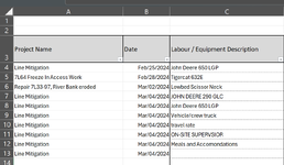
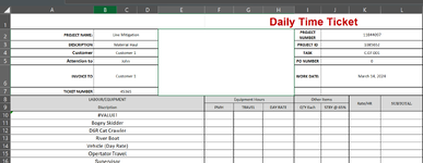
I find myself needing some help on a problem I am having. I am looking to get a list from my Entry tab that meets two criteria, the two criteria are the date and Project Name. I am trying to use Index Match but have not yet gotten very far. Can anyone help?

Thanks in advance

 

[Bob_ipc]

In your summary, your workday is 3/14. There's nothing in the entry tab that has the date 3/14. If you're certain that the references are correct the formatting isn't an issue, and there's nothing to return then try this...

=FILTER(Entry!C4:C13,(Entry!A4:A13=B2)*(Entry!B4:B13=J6),"Not found")

Hey, yes I did see that I had the incorrect date there and had change it to 3/04, Now when I put in =FILTER(Entry!C4:C13,(Entry!A4:A13=B2)*(Entry!B4:B13=J6),"Not found") it returns "Not Found"

 

[Bob_ipc]

Yes...that's the point about the cell address. The image doesn't tell us if the project name is in B2 or C2...and date in J6 or K6. You may need to adjust those references in the formula to point to the correct cell(s).

Ah gotcha that makes sense, so I changed it to references to make it look like this =FILTER('Entry'!C4:C400,('Entry'!A4:A400=B2:D2)*('Entry'!B4=J6:L6),"Not found") but now it is returning #VALUE!

 

[KRice]

No...not B2:D2 or J6:L6. Should be a single cell reference just like @Cubist had, although maybe its not B2...could be C2. You'll need to check which cell actually holds the values of interest.

I suspect @Cubist's point about the date format may be the issue. The dates in column B have an unusual format mmm/dd/yyyy. Reformat one of those date entries as a number, not a date, and see if it returns a numeric value around 45355.

 

[Bob_ipc]

No...not B2:D2 or J6:L6. Should be a single cell reference just like @Cubist had, although maybe its not B2...could be C2. You'll need to check which cell actually holds the values of interest.

I suspect @Cubist's point about the date format may be the issue. The dates in column B have an unusual format mmm/dd/yyyy. Reformat one of those date entries as a number, not a date, and see if it returns a numeric value around 45355.

Ok so I tried B2, C2, D2 as well as J6, K6, L6 and that didn't do the trick. And when I change the date format to General it does give me a number of 45355. I have also reformatted the date to 3/4/2024. Still no change

 

[KRice]

In some empty cell on the worksheet, type =B2 and let us know if the project name "Line mitigation" appears. Similarly, type =J6 and tell us what you get.

 

[Bob_ipc]

In some empty cell on the worksheet, type =B2 and let us know if the project name "Line mitigation" appears. Similarly, type =J6 and tell us what you get.

So B2 returns Line Mitigation and J6 returns 3/4/2024, so I have B2 and J6 in the formula.

 

[Cubist]

Book2.xlsx
	A	B	C
1
2
3	Project Name	Date	Equipment
4	Project A	Feb/25/2024	Chain saw
5	Project B	Feb/28/2024	John Deer
6	Project C	Mar/2/2024	Vechicle
7	Project A	Mar/4/2024	Crew truck
8	Project A	Mar/4/2024	travel rate
9	Project A	Mar/4/2024	On-site
10	Project A	Mar/4/2024	Meals
11	Project A	Mar/4/2024
Entry

Book2.xlsx
	A	B	C	D	E	F	G	H	I	J
2	Project Name	Project A
3
4
5
6									Work Date	March 04,2024
7
8	Equipment
9	Crew truck
10	travel rate
11	On-site
12	Meals
13	0
14
15
Summary

Cell Formulas
Range	Formula
A9:A13	A9	=FILTER(Entry!C4:C11,(Summary!$B$2=Entry!A4:A11)*(Summary!$J$6=Entry!B4:B11),"Not found")
Dynamic array formulas.

 

[KRice]

Somewhere on the data worksheet (the "Entry tab")...out to the right in some empty column, in row 4, enter:

=A4:A13="Line Mitigation"

...and let us know if you see a vertical array of TRUEs and FALSEs...and those correspond correctly to the data table.

 

[Bob_ipc]

Book2.xlsx
	A	B	C
1
2
3	Project Name	Date	Equipment
4	Project A	Feb/25/2024	Chain saw
5	Project B	Feb/28/2024	John Deer
6	Project C	Mar/2/2024	Vechicle
7	Project A	Mar/4/2024	Crew truck
8	Project A	Mar/4/2024	travel rate
9	Project A	Mar/4/2024	On-site
10	Project A	Mar/4/2024	Meals
11	Project A	Mar/4/2024
Entry

Book2.xlsx
	A	B	C	D	E	F	G	H	I	J
2	Project Name	Project A
3
4
5
6									Work Date	March 04,2024
7
8	Equipment
9	Crew truck
10	travel rate
11	On-site
12	Meals
13	0
14
15
Summary

Cell Formulas
Range	Formula
A9:A13	A9	=FILTER(Entry!C4:C11,(Summary!$B$2=Entry!A4:A11)*(Summary!$J$6=Entry!B4:B11),"Not found")
Dynamic array formulas.

THIS WORKS!! so awesome! Thank you!

 

[KRice]

That still doesn't explain why @Cubist's formula in post #2 wasn't working for you. You don't need to specify the worksheet name when the formula resides on that same worksheet.

=FILTER(Entry!C4:C13,(Entry!A4:A13=B2)*(Entry!B4:B13=J6),"Not found")

...should still work.