Linking Cells to Calculate - IF function?

[Sambrowne]

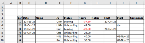
I have a spreadsheet with one sheet that has fixed cells for employee hours and another sheet where I enter leavers and joiners. This latter sheet is not fixed and is free text albeit with drop down occupation codes that are the same between the two sheets. What I want to do is enter a leaver or a joiner on one sheet and have it update the main hours sheet but because the second sheet is effectively free text I can't see how to do it. One cell can't be linked permanently to the other. My gut feeling is through the job codes. So when someone enters leaving hours for UNM (Unit Manager) it links to the other sheet through UNM and updates the hours accordingly. I think this is an IF function but I'm a bit stumped. Thanks!

 

[dreid1011]

No, that doesn't really help much. The formula I provided should go into cell H5, drag it over to I5, then drag both columns down to the end of your data. If that does not provide the results you are seeking, then we can take another look. I was able to return 44 for line 3 with UNM, but I don't know where you're getting the other values in columns H:I, unless they don't have anything to do with it.

 

[Sambrowne]

I can't get it to work at all, I paste it into H5, to drag it across and then I get 'Cannot find "Free, fixed codes". Copy from:' What am I doing wrong?

 

[dreid1011]

I can't get it to work at all, I paste it into H5, to drag it across and then I get 'Cannot find "Free, fixed codes". Copy from:' What am I doing wrong?

It must be the sheet name then. I assumed "Free, fixed codes" was your sheet name for the second sheet based on your screenshot names. If that is incorrect, change that text in the formula to the name of your second sheet.

 

[Sambrowne]

D'oh! Ok, got it to work but I had a formula in J5 (=F5+I5-(G5+H5) to net the onboarding/leaving to give me a final figure. If the cells have no data I get a value error. Not sure where to go now? Thanks for your patience and help with this I really appreciate it, I would never have got this far!

Book1.xlsx
	A	B	C	D	E	F	G	H	I	J	K
2			Ramp Scenarios
3			Careblox		Use drop down		0%
4		Ser	Role	JC	R3	Ramp + flex	Contracted	Onboarding	Leaving	Recruit	Comments
5		1	DM	DEP	40	40	40			#VALUE!
6		2	Adv Senior Carer	ADC	40	40	0			#VALUE!
7		3	Unit Mgr	UNM	101.25	101.25	39.75	44	37.5	55.00
8		4	SCR Days	SCR	315	315	198.75			#VALUE!	#VALUE!
9		5	CAR Days	CAR	462	462	529		20	#VALUE!
10		6	SCR Nights	SCR	236.25	236.25	122			#VALUE!
11		7	CAR Nights	CAR	231	231	308		20	#VALUE!
12		8	Maintenance	MAI	37.5	37.5	37.5			#VALUE!
13		9	Gardener	MAI	25	25	0			#VALUE!
14		10	Admin	ADM	40	40	37.5			#VALUE!
15		18	Reception	REC	77	77	55.5			#VALUE!
16		11	Head Chef	HCF	40	40	40			#VALUE!
17		12	Sous Chef	SOU	40	40	0			#VALUE!
18		13	Commis Chef	CHE	25	25	0	24		#VALUE!
19		14	Kitchen Asst	KIT	80	80	80			#VALUE!
20		15	Head Housekeeper	SHO	37.5	37.5	37.5			#VALUE!
21		16	Housekeepers and Laundry Consolidated	HOU	120	120	151			31.00
22		17	Housekeeper	HOU	62.5	62.5	121			#VALUE!	Careblox data includes laundry
23		18	Laundry Asst	LAU	58	58	30			#VALUE!	See note above
24		19	Act Coord	HRL	38	38	0	40		#VALUE!
25		20	Act Asst	RAL	33	33	0	30		#VALUE!
26		21	Staff Wellbeing		4	4	0			#VALUE!
27		22	Driver	DRV	14	14	0			#VALUE!
28						0
29		23	Totals		2036.5	2036.5	1676.5	138	77.5	#VALUE!
Ramps

Cell Formulas
Range	Formula
H5:I27	H5	=XLOOKUP($D5&H$4,'Onboarders and Leavers'!$E$5:$E$25&'Onboarders and Leavers'!$F$5:$F$25,'Onboarders and Leavers'!$G$5:$G$25,"")
J22:J27,J5:J20	J5	=F5+I5-(G5+H5)
K8	K8	=(J8+J7)
E5	E5	=IF(E4="","",IF(E4="R1",40,IF(E4="R2",40,IF(E4="R3",40,IF(E4="R4",40,IF(E4="Ramp",0,"Check Entry"))))))
E6	E6	=IF(E4="","",IF(E4="R1",40,IF(E4="R2",40,IF(E4="R3",40,IF(E4="R4",40,IF(E4="Ramp",0,"Check Entry"))))))
E7	E7	=IF(E4="","",IF(E4="R1",101.25,IF(E4="R2",101.25,IF(E4="R3",101.25,IF(E4="R4",101.25,IF(E4="Ramp",0,"Check Entry"))))))
E8	E8	=IF(E4="","",IF(E4="R1",157.5,IF(E4="R2",236.25,IF(E4="R3",315,IF(E4="R4",315,IF(E4="Ramp",0,"Check Entry"))))))
E9	E9	=IF(E4="","",IF(E4="R1",308,IF(E4="R2",385,IF(E4="R3",462,IF(E4="R4",539,IF(E4="Ramp",0,"Check Entry"))))))
E10	E10	=IF(E4="","",IF(E4="R1",157.5,IF(E4="R2",236.25,IF(E4="R3",236.25,IF(E4="R4",315,IF(E4="Ramp",0,"Check Entry"))))))
E11	E11	=IF(E4="","",IF(E4="R1",154,IF(E4="R2",154,IF(E4="R3",231,IF(E4="R4",231,IF(E4="Ramp",0,"Check Entry"))))))
E12	E12	=IF(E4="","",IF(E4="R1",37.5,IF(E4="R2",37.5,IF(E4="R3",37.5,IF(E4="R4",37.5,IF(E4="Ramp",0,"Check Entry"))))))
E13	E13	=IF(E4="","",IF(E4="R1",0,IF(E4="R2",25,IF(E4="R3",25,IF(E4="R4",25,IF(E4="Ramp",0,"Check Entry"))))))
E14	E14	=IF(E4="","",IF(E4="R1",40,IF(E4="R2",40,IF(E4="R3",40,IF(E4="R4",40,IF(E4="Ramp",0,"Check Entry"))))))
E15	E15	=IF(E4="","",IF(E4="R1",77,IF(E4="R2",77,IF(E4="R3",77,IF(E4="R4",77,IF(E4="Ramp",0,"Check Entry"))))))
E16	E16	=IF(E4="","",IF(E4="R1",40,IF(E4="R2",40,IF(E4="R3",40,IF(E4="R4",40,IF(E4="Ramp",0,"Check Entry"))))))
E17	E17	=IF(E4="","",IF(E4="R1",40,IF(E4="R2",40,IF(E4="R3",40,IF(E4="R4",40,IF(E4="Ramp",0,"Check Entry"))))))
E18	E18	=IF(E4="","",IF(E4="R1",0,IF(E4="R2",25,IF(E4="R3",25,IF(E4="R4",25,IF(E4="Ramp",0,"Check Entry"))))))
E19	E19	=IF(E4="","",IF(E4="R1",80,IF(E4="R2",80,IF(E4="R3",80,IF(E4="R4",80,IF(E4="Ramp",0,"Check Entry"))))))
E21	E21	=IF(E4="","",IF(E4="R1",78.5,IF(E4="R2",88.5,IF(E4="R3",120,IF(E4="R4",134,IF(E4="Ramp",0,"Check Entry"))))))
E22	E22	=IF(E4="","",IF(E4="R1",38.5,IF(E4="R2",48.5,IF(E4="R3",62.5,IF(E4="R4",76.5,IF(E4="Ramp",0,"Check Entry"))))))
E23	E23	=IF(E4="","",IF(E4="R1",40,IF(E4="R2",40,IF(E4="R3",58,IF(E4="R4",58,IF(E4="Ramp",0,"Check Entry"))))))
E24	E24	=IF(E4="","",IF(E4="R1",38,IF(E4="R2",38,IF(E4="R3",38,IF(E4="R4",38,IF(E4="Ramp",0,"Check Entry"))))))
E25	E25	=IF(E4="","",IF(E4="R1",17,IF(E4="R2",17,IF(E4="R3",33,IF(E4="R4",33,IF(E4="Ramp",0,"Check Entry"))))))
E26	E26	=IF(E4="","",IF(E4="R1",4,IF(E4="R2",4,IF(E4="R3",4,IF(E4="R4",4,IF(E4="Ramp",0,"Check Entry"))))))
E27	E27	=IF(E4="","",IF(E4="R1",14,IF(E4="R2",14,IF(E4="R3",14,IF(E4="R4",14,IF(E4="Ramp",0,"Check Entry"))))))
F5:F29	F5	=(E5*$G$3)+E5
E29,G29:J29	E29	=SUM(E5:E21)+SUM(E24:E27)

Cells with Data Validation
Cell	Allow	Criteria
E4	List	Ramp, R1, R2, R3, R4

Book1.xlsx
	B	C	D	E	F	G	H	I	J	K
4	Ser	Date	Name	JC	Status	Hours	Notice	LWD	Start	Comments
5	1	22-Sep-23	Lady Alice	UNM	Leaving	37.50		22-Oct-23
6	2	18-Oct-23	Lord Bulbous	UNM	Onboarding	44.00			tbc
7	3	19-Oct-23	Sir Chav	CAR	Leaving	20.00		20-Oct-23
8	4	9-Oct-23	Major ****	CHE	Onboarding	24.00
9	5		Mr Egg	HRL	Onboarding	40.00			2-Nov-23
10	6		Mrs Flub	RAL	Onboarding	30.00			2-Nov-23
11	7
12	8
13	9
14	10
15	11
16	12
17	13
18	14
19	15
20	16
21	17
22	18
23	19
24	20
25	21
Onboarders and Leavers

Cells with Data Validation
Cell	Allow	Criteria
E5:E25	List	ADM, ADC, CAR, CHE, DEP, DRV, HOU, HCF, HRL, KIT, LAU, MAI, MAN, REC, RAL, SCR, SHO, SOU, UNM
F5:F25	List	Onboarding, Leaving

 

[dreid1011]

You could wrap the J5 formula in IFERROR like this:

=IFERROR(F5+I5-(G5+H5),"")

 

[Sambrowne]

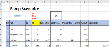
Cheers, that worked - sort of! If you look at row 10 on the first sheet (Ramps) there should be 116.25 in there but the LOOKUP has wiped out that formula (even though it's still in the cell) and the IFERROR doesn't resolve it either.

 

[dreid1011]

Which row 10 are you referring to? Row 10 for SCR Nights, or SER 10 for Admin?

 

[Sambrowne]

Sorry, SCR nights.

 

[dreid1011]

And which cell should have 116.25?

 

[Sambrowne]

Sorry, should be 114.25 (not 116.25) in cell J10.