SophieYaldwyn
New Member
- Joined
- Sep 13, 2022
- Messages
- 9
- Office Version
- 365
- Platform
- Windows
Hi all,
I am trying to link separate workbooks-not-worksheets that are yet to be created - these would be workbooks created in the future using templates, and the destination workbook I am working in will be a master template as well. This is for a project for study and I have really hit a roadblock here and perhaps thinking I need to completely re-think the entire first workbook I have created. For full information, the study question reads:
"Create a series of Excel spreadsheets to demonstrate the skills you learned in this module.
You will need to demonstrate your ability to design a group of spreadsheets that:
Example:
A friend knows you have a good understanding of Excel.
He would like you to help him with his business. He wants to keep a spreadsheet for each month’s sales. He has five sales staff and would like to record the daily sales figure. He wants to see a monthly total for each person and a daily sales total. He would also like an average daily sale, the lowest sales figure, and the highest sales figure for each day. The data should have highlighting to show figures below the daily average and figures above the average. There should be a separate worksheet that shows a commission figure for each salesperson daily. He pays each person a flat 15% of everything they sell as a commission.
He thinks a template for the above spreadsheet would help him create a new spreadsheet every month.
Then he would like a master spreadsheet that shows each person’s monthly sales figure. He would like to have an annual total for each and a grand total. He would like a chart showing each person by month and another chart that shows each person’s annual sales figure as a part of the total sales figure."
Is what I am trying to achieve something that is possible?
I have been trying to have a reference cell in the master workbook that shows the workbook-to-be-referenced file name that can then be referenced in the formulae throughout the workbook. So as the new workbooks are created, that reference cell can be edited to contain the new workbook name, which would then automatically adjust content in all the formulae throughout the workbook to create the correct path.
I keep coming up with a File Name Syntax error though when trying to reference that reference cell (I3) in creating the new formula rather than clicking on a cell in the separate workbook.
Hopefully this makes sense and someone is able to lend some expertise. I have attached all workbooks and worksheets below for reference and a screenshot of the error.
Thankyou!
Sophie
Workbook 1, sheet 1:
Workbook 1 Sheet 2:
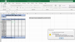
Workbook 2, Sheet 1 - Where I am trying to create the link using cell I3 as a reference within a cell link such as cell B5 but not manually input.
I am trying to link separate workbooks-not-worksheets that are yet to be created - these would be workbooks created in the future using templates, and the destination workbook I am working in will be a master template as well. This is for a project for study and I have really hit a roadblock here and perhaps thinking I need to completely re-think the entire first workbook I have created. For full information, the study question reads:
"Create a series of Excel spreadsheets to demonstrate the skills you learned in this module.
You will need to demonstrate your ability to design a group of spreadsheets that:
- have a link between one spreadsheet and another
- demonstrates conditional formatting
- use at least three functions from Excel and one formula you create
- has at least one macro
- uses a template you created to produce new workbooks
- uses charts to help analyse data
Example:
A friend knows you have a good understanding of Excel.
He would like you to help him with his business. He wants to keep a spreadsheet for each month’s sales. He has five sales staff and would like to record the daily sales figure. He wants to see a monthly total for each person and a daily sales total. He would also like an average daily sale, the lowest sales figure, and the highest sales figure for each day. The data should have highlighting to show figures below the daily average and figures above the average. There should be a separate worksheet that shows a commission figure for each salesperson daily. He pays each person a flat 15% of everything they sell as a commission.
He thinks a template for the above spreadsheet would help him create a new spreadsheet every month.
Then he would like a master spreadsheet that shows each person’s monthly sales figure. He would like to have an annual total for each and a grand total. He would like a chart showing each person by month and another chart that shows each person’s annual sales figure as a part of the total sales figure."
Is what I am trying to achieve something that is possible?
I have been trying to have a reference cell in the master workbook that shows the workbook-to-be-referenced file name that can then be referenced in the formulae throughout the workbook. So as the new workbooks are created, that reference cell can be edited to contain the new workbook name, which would then automatically adjust content in all the formulae throughout the workbook to create the correct path.
I keep coming up with a File Name Syntax error though when trying to reference that reference cell (I3) in creating the new formula rather than clicking on a cell in the separate workbook.
Hopefully this makes sense and someone is able to lend some expertise. I have attached all workbooks and worksheets below for reference and a screenshot of the error.
Thankyou!
Sophie
Workbook 1, sheet 1:
| ProjectBSBTEC402P1.xlsm | |||||||||||
|---|---|---|---|---|---|---|---|---|---|---|---|
| A | B | C | D | E | F | G | H | I | |||
| 1 | Monthly Sales Figures: Business Name | ||||||||||
| 2 | Month | 2 | Above Average | Below Average | Highest Figure | Lowest Figure | |||||
| 3 | Year | 2022 | Legend: | ||||||||
| 4 | Leap Year? | No | |||||||||
| 5 | Date | Day | Person 1 | Person 2 | Person 3 | Person 4 | Person 5 | Average Daily Sale Total | Overall Daily Sales Total | ||
| 6 | 1 | Tue | $ 123.00 | $ 123.00 | $ 123.00 | ||||||
| 7 | 2 | Wed | $ 798.00 | $ 798.00 | $ 798.00 | ||||||
| 8 | 3 | Thu | $ 23,545.00 | $ 7,856.00 | $ 15,700.50 | $ 31,401.00 | |||||
| 9 | 4 | Fri | $ 987.00 | $ 987.00 | $ 987.00 | ||||||
| 10 | 5 | Sat | $ 3,453.00 | $ 5,668.00 | $ 4,560.50 | $ 9,121.00 | |||||
| 11 | 6 | Sun | $ 3,246.00 | $ 3,246.00 | $ 3,246.00 | ||||||
| 12 | 7 | Mon | |||||||||
| 13 | 8 | Tue | |||||||||
| 14 | 9 | Wed | |||||||||
| 15 | 10 | Thu | |||||||||
| 16 | 11 | Fri | |||||||||
| 17 | 12 | Sat | |||||||||
| 18 | 13 | Sun | |||||||||
| 19 | 14 | Mon | |||||||||
| 20 | 15 | Tue | |||||||||
| 21 | 16 | Wed | |||||||||
| 22 | 17 | Thu | |||||||||
| 23 | 18 | Fri | |||||||||
| 24 | 19 | Sat | |||||||||
| 25 | 20 | Sun | |||||||||
| 26 | 21 | Mon | |||||||||
| 27 | 22 | Tue | |||||||||
| 28 | 23 | Wed | |||||||||
| 29 | 24 | Thu | |||||||||
| 30 | 25 | Fri | |||||||||
| 31 | 26 | Sat | |||||||||
| 32 | 27 | Sun | |||||||||
| 33 | 28 | Mon | |||||||||
| 34 | #VALUE! | ||||||||||
| 35 | #VALUE! | ||||||||||
| 36 | #VALUE! | ||||||||||
| 37 | Monthly Total | $ 28,906.00 | $ 16,770.00 | $ 45,676.00 | |||||||
| 38 | Overall Daily Sale Average | $ 4,235.83 | |||||||||
MonthlySalesFigures | |||||||||||
| Cell Formulas | ||
|---|---|---|
| Range | Formula | |
| B4 | B4 | =IF(MONTH(DATE(B3,2,29))=2,"Yes","No") |
| H6:H20,H25:H36 | H6 | =IFERROR(AVERAGE(C6:G6),"") |
| B6:B36 | B6 | =DATE($B$3,$B$2,$A6) |
| A34 | A34 | =IF(OR(B2=1,B2=3,B2=4,B2=5,B2=6,B2=7,B2=8,B2=9,B2=10,B2=11,B2=12,B4="Yes"), "29", "") |
| A35 | A35 | =IF(B2=2,"","30") |
| A36 | A36 | =IF(OR(B2=1,B2=3,B2=5,B2=7,B2=8,B2=10,B2=12),"31","") |
| C37:G37,I37 | C37 | =IF(SUM(C6:C36)=0,"",SUM(C6:C36)) |
| I6:I36 | I6 | =IF(SUM(C6:G6)=0,"",SUM(C6:G6)) |
| H38 | H38 | =IFERROR(AVERAGEIF(H6:H36,"<>-"),"") |
| Cells with Conditional Formatting | ||||
|---|---|---|---|---|
| Cell | Condition | Cell Format | Stop If True | |
| C36:G36 | Cell Value | top 1 bottom values | text | NO |
| C36:G36 | Cell Value | top 1 values | text | NO |
| C36:G36 | Cell Value | below average | text | NO |
| C36:G36 | Cell Value | above average | text | NO |
| C35:G35 | Cell Value | top 1 bottom values | text | NO |
| C35:G35 | Cell Value | top 1 values | text | NO |
| C35:G35 | Cell Value | below average | text | NO |
| C35:G35 | Cell Value | above average | text | NO |
| C34:G34 | Cell Value | top 1 bottom values | text | NO |
| C34:G34 | Cell Value | top 1 values | text | NO |
| C34:G34 | Cell Value | below average | text | NO |
| C34:G34 | Cell Value | above average | text | NO |
| C33:G33 | Cell Value | top 1 bottom values | text | NO |
| C33:G33 | Cell Value | top 1 values | text | NO |
| C33:G33 | Cell Value | below average | text | NO |
| C33:G33 | Cell Value | above average | text | NO |
| C32:G32 | Cell Value | top 1 bottom values | text | NO |
| C32:G32 | Cell Value | top 1 values | text | NO |
| C32:G32 | Cell Value | below average | text | NO |
| C32:G32 | Cell Value | above average | text | NO |
| C31:G31 | Cell Value | top 1 bottom values | text | NO |
| C31:G31 | Cell Value | top 1 values | text | NO |
| C31:G31 | Cell Value | below average | text | NO |
| C31:G31 | Cell Value | above average | text | NO |
| C30:G30 | Cell Value | top 1 bottom values | text | NO |
| C30:G30 | Cell Value | top 1 values | text | NO |
| C30:G30 | Cell Value | below average | text | NO |
| C30:G30 | Cell Value | above average | text | NO |
| C29:G29 | Cell Value | top 1 bottom values | text | NO |
| C29:G29 | Cell Value | top 1 values | text | NO |
| C29:G29 | Cell Value | below average | text | NO |
| C29:G29 | Cell Value | above average | text | NO |
| C28:G28 | Cell Value | top 1 bottom values | text | NO |
| C28:G28 | Cell Value | top 1 values | text | NO |
| C28:G28 | Cell Value | below average | text | NO |
| C28:G28 | Cell Value | above average | text | NO |
| C27:G27 | Cell Value | top 1 bottom values | text | NO |
| C27:G27 | Cell Value | top 1 values | text | NO |
| C27:G27 | Cell Value | below average | text | NO |
| C27:G27 | Cell Value | above average | text | NO |
| C25:G25 | Cell Value | top 1 bottom values | text | NO |
| C25:G25 | Cell Value | top 1 values | text | NO |
| C25:G25 | Cell Value | below average | text | NO |
| C25:G25 | Cell Value | above average | text | NO |
| C23:G23 | Cell Value | top 1 bottom values | text | NO |
| C23:G23 | Cell Value | top 1 values | text | NO |
| C23:G23 | Cell Value | below average | text | NO |
| C23:G23 | Cell Value | above average | text | NO |
| C24:G24 | Cell Value | top 1 bottom values | text | NO |
| C24:G24 | Cell Value | top 1 values | text | NO |
| C24:G24 | Cell Value | below average | text | NO |
| C24:G24 | Cell Value | above average | text | NO |
| C26:G26 | Cell Value | top 1 bottom values | text | NO |
| C26:G26 | Cell Value | top 1 values | text | NO |
| C26:G26 | Cell Value | below average | text | NO |
| C26:G26 | Cell Value | above average | text | NO |
| C22:G22 | Cell Value | top 1 bottom values | text | NO |
| C22:G22 | Cell Value | top 1 values | text | NO |
| C22:G22 | Cell Value | below average | text | NO |
| C22:G22 | Cell Value | above average | text | NO |
| C21:G21 | Cell Value | top 1 bottom values | text | NO |
| C21:G21 | Cell Value | top 1 values | text | NO |
| C21:G21 | Cell Value | below average | text | NO |
| C21:G21 | Cell Value | above average | text | NO |
| C20:G20 | Cell Value | top 1 bottom values | text | NO |
| C20:G20 | Cell Value | top 1 values | text | NO |
| C20:G20 | Cell Value | below average | text | NO |
| C20:G20 | Cell Value | above average | text | NO |
| C19:G19 | Cell Value | top 1 bottom values | text | NO |
| C19:G19 | Cell Value | top 1 values | text | NO |
| C19:G19 | Cell Value | below average | text | NO |
| C19:G19 | Cell Value | above average | text | NO |
| C18:G18 | Cell Value | top 1 bottom values | text | NO |
| C18:G18 | Cell Value | top 1 values | text | NO |
| C18:G18 | Cell Value | below average | text | NO |
| C18:G18 | Cell Value | above average | text | NO |
| C17:G17 | Cell Value | top 1 bottom values | text | NO |
| C17:G17 | Cell Value | top 1 values | text | NO |
| C17:G17 | Cell Value | below average | text | NO |
| C17:G17 | Cell Value | above average | text | NO |
| C16:G16 | Cell Value | top 1 bottom values | text | NO |
| C16:G16 | Cell Value | top 1 values | text | NO |
| C16:G16 | Cell Value | below average | text | NO |
| C16:G16 | Cell Value | above average | text | NO |
| C15:G15 | Cell Value | top 1 bottom values | text | NO |
| C15:G15 | Cell Value | top 1 values | text | NO |
| C15:G15 | Cell Value | below average | text | NO |
| C15:G15 | Cell Value | above average | text | NO |
| C14:G14 | Cell Value | top 1 bottom values | text | NO |
| C14:G14 | Cell Value | top 1 values | text | NO |
| C14:G14 | Cell Value | below average | text | NO |
| C14:G14 | Cell Value | above average | text | NO |
| C13:G13 | Cell Value | top 1 bottom values | text | NO |
| C13:G13 | Cell Value | top 1 values | text | NO |
| C13:G13 | Cell Value | below average | text | NO |
| C13:G13 | Cell Value | above average | text | NO |
| C10:G10 | Cell Value | top 1 bottom values | text | NO |
| C10:G10 | Cell Value | top 1 values | text | NO |
| C10:G10 | Cell Value | below average | text | NO |
| C10:G10 | Cell Value | above average | text | NO |
| C8:G8 | Cell Value | top 1 bottom values | text | NO |
| C8:G8 | Cell Value | top 1 values | text | NO |
| C8:G8 | Cell Value | below average | text | NO |
| C8:G8 | Cell Value | above average | text | NO |
| C9:G9 | Cell Value | top 1 bottom values | text | NO |
| C9:G9 | Cell Value | top 1 values | text | NO |
| C9:G9 | Cell Value | below average | text | NO |
| C9:G9 | Cell Value | above average | text | NO |
| C12:G12 | Cell Value | top 1 bottom values | text | NO |
| C12:G12 | Cell Value | top 1 values | text | NO |
| C12:G12 | Cell Value | below average | text | NO |
| C12:G12 | Cell Value | above average | text | NO |
| C11:G11 | Cell Value | top 1 bottom values | text | NO |
| C11:G11 | Cell Value | top 1 values | text | NO |
| C11:G11 | Cell Value | below average | text | NO |
| C11:G11 | Cell Value | above average | text | NO |
| C7:G7 | Cell Value | top 1 bottom values | text | NO |
| C7:G7 | Cell Value | top 1 values | text | NO |
| C6:G6 | Cell Value | top 1 bottom values | text | NO |
| C6:G6 | Cell Value | top 1 values | text | NO |
| C7:G7 | Cell Value | below average | text | NO |
| C7:G7 | Cell Value | above average | text | NO |
| C6:G6 | Cell Value | above average | text | NO |
| C6:G6 | Cell Value | below average | text | NO |
| A34 | Cell | contains an error | text | NO |
| B34:B36 | Cell | contains an error | text | NO |
| Cells with Data Validation | ||
|---|---|---|
| Cell | Allow | Criteria |
| B2 | List | 1,2,3,4,5,6,7,8,9,10,11,12 |
| B3 | List | 2022,2023,2024,2025,2026,2027,2028,2029,2030,2031,2032,2033,2034,2035,2036,2037,2038,2039,2040,2041,2042,2043,2044,2045,2046,2047,2048,2049,2050,2051,2052,2053,2054,2055,2056,2057,2058,2059,2060,2061,2062,2063,2064,2065,2066,2067,2068,2069,2070,2071,2072 |
Workbook 1 Sheet 2:
| ProjectBSBTEC402P1.xlsm | |||||||||
|---|---|---|---|---|---|---|---|---|---|
| A | B | C | D | E | F | G | |||
| 1 | Monthly Commission Figures: Business Name | ||||||||
| 2 | Month | 2 | |||||||
| 3 | Year | 2022 | Commission Rate: | 15% | |||||
| 4 | Leap Year? | No | |||||||
| 5 | Date | Day | Person 1 | Person 2 | Person 3 | Person 4 | Person 5 | ||
| 6 | 1 | Tue | $ 18.45 | ||||||
| 7 | 2 | Wed | $ 119.70 | ||||||
| 8 | 3 | Thu | $3,531.75 | $1,178.40 | |||||
| 9 | 4 | Fri | $ 148.05 | ||||||
| 10 | 5 | Sat | $ 517.95 | $ 850.20 | |||||
| 11 | 6 | Sun | $ 486.90 | ||||||
| 12 | 7 | Mon | |||||||
| 13 | 8 | Tue | |||||||
| 14 | 9 | Wed | |||||||
| 15 | 10 | Thu | |||||||
| 16 | 11 | Fri | |||||||
| 17 | 12 | Sat | |||||||
| 18 | 13 | Sun | |||||||
| 19 | 14 | Mon | |||||||
| 20 | 15 | Tue | |||||||
| 21 | 16 | Wed | |||||||
| 22 | 17 | Thu | |||||||
| 23 | 18 | Fri | |||||||
| 24 | 19 | Sat | |||||||
| 25 | 20 | Sun | |||||||
| 26 | 21 | Mon | |||||||
| 27 | 22 | Tue | |||||||
| 28 | 23 | Wed | |||||||
| 29 | 24 | Thu | |||||||
| 30 | 25 | Fri | |||||||
| 31 | 26 | Sat | |||||||
| 32 | 27 | Sun | |||||||
| 33 | 28 | Mon | |||||||
| 34 | #VALUE! | ||||||||
| 35 | #VALUE! | ||||||||
| 36 | #VALUE! | ||||||||
| 37 | Monthly Total | $4,335.90 | $2,515.50 | ||||||
CommissionCalculations | |||||||||
| Cell Formulas | ||
|---|---|---|
| Range | Formula | |
| B2:B3 | B2 | =MonthlySalesFigures!B2 |
| B4 | B4 | =IF(MONTH(DATE(B3,2,29))=2,"Yes","No") |
| C6:G36 | C6 | =IF(MonthlySalesFigures!C6*$G$3=0,"",MonthlySalesFigures!C6*$G$3) |
| C37:G37 | C37 | =IF(SUM(C6:C36)=0,"",SUM(C6:C36)) |
| B6:B36 | B6 | =DATE($B$3,$B$2,$A6) |
| A34 | A34 | =IF(OR(B2=1,B2=3,B2=4,B2=5,B2=6,B2=7,B2=8,B2=9,B2=10,B2=11,B2=12,B4="Yes"), "29", "") |
| A35 | A35 | =IF(B2=2,"","30") |
| A36 | A36 | =IF(OR(B2=1,B2=3,B2=5,B2=7,B2=8,B2=10,B2=12),"31","") |
| Cells with Conditional Formatting | ||||
|---|---|---|---|---|
| Cell | Condition | Cell Format | Stop If True | |
| A34 | Cell | contains an error | text | NO |
| B34:B36 | Cell | contains an error | text | NO |
| Cells with Data Validation | ||
|---|---|---|
| Cell | Allow | Criteria |
| B2 | List | 1,2,3,4,5,6,7,8,9,10,11,12 |
| B3 | List | 2022,2023,2024,2025,2026,2027,2028,2029,2030,2031,2032,2033,2034,2035,2036,2037,2038,2039,2040,2041,2042,2043,2044,2045,2046,2047,2048,2049,2050,2051,2052,2053,2054,2055,2056,2057,2058,2059,2060,2061,2062,2063,2064,2065,2066,2067,2068,2069,2070,2071,2072 |
Workbook 2, Sheet 1 - Where I am trying to create the link using cell I3 as a reference within a cell link such as cell B5 but not manually input.
| Project BSBTEC402 P21.xlsx | |||||||||||
|---|---|---|---|---|---|---|---|---|---|---|---|
| A | B | C | D | E | F | G | H | I | |||
| 1 | Individual Sales Figure Totals | ||||||||||
| 2 | Year | ||||||||||
| 3 | File name of source workbook | ProjectBSBTEC402P1.xlsm | |||||||||
| 4 | Month | Person 1 | Person 2 | Person 3 | Person 4 | Person 5 | |||||
| 5 | January | $ 28,906.00 | |||||||||
| 6 | February | ||||||||||
| 7 | March | ||||||||||
| 8 | April | ||||||||||
| 9 | May | ||||||||||
| 10 | June | ||||||||||
| 11 | July | ||||||||||
| 12 | August | ||||||||||
| 13 | September | ||||||||||
| 14 | October | ||||||||||
| 15 | November | ||||||||||
| 16 | December | ||||||||||
| 17 | Annual Total | ||||||||||
| 18 | Annual Grand Total | ||||||||||
Sheet1 | |||||||||||
| Cell Formulas | ||
|---|---|---|
| Range | Formula | |
| B5 | B5 | =[ProjectBSBTEC402P1.xlsm]MonthlySalesFigures!$C$37 |