look up with date ranges

ExcelNewbie2020 · Mar 25, 2023

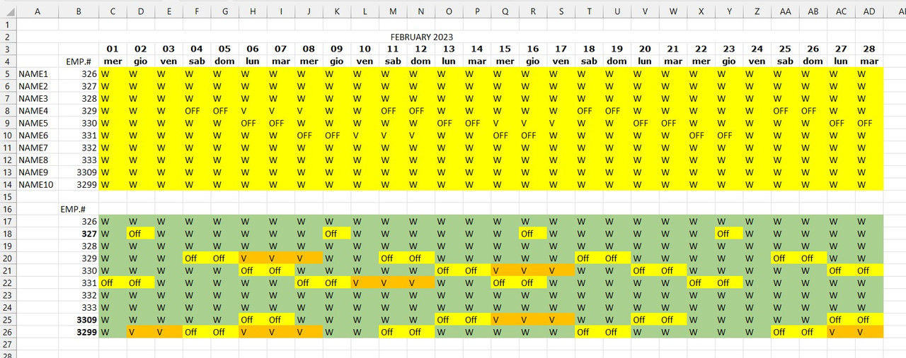
i have this table in sheet 1 and sheet 2..I need a formula in sheet 1 (in yellow). that will auto populate based on the data in sheet 2 (in blue). wherein sheet 2 is the input table. I will input the "OFF" schedule that should appear in sheet 1... while the vacation (from start to end) should populate once the status is "OK"..Otherwise, "W" should appear.

4_Must-Have_AI_Tools (version 1).xlsb

A

B

C

D

E

F

G

H

I

J

K

L

M

N

O

P

Q

R

S

T

U

V

W

X

Y

Z

AA

AB

AC

AD

AE

AF

AG

AH

AI

AJ

AK

AL

1

SHEET 1

SHEET 2

2

FEBRUARY 2023

VACATION (VL)

3

01

02

03

04

05

06

07

08

09

10

11

12

13

14

15

16

17

18

19

20

21

22

23

24

25

26

27

28

EMP.#

OFF

START

END

STATUS

4

EMP.#

Wed

Thu

Fri

Sat

Sun

Mon

Tue

Wed

Thu

Fri

Sat

Sun

Mon

Tue

Wed

Thu

Fri

Sat

Sun

Mon

Tue

Wed

Thu

Fri

Sat

Sun

Mon

Tue

NAME4

329

Sat

Sun

06-02-23

08-02-23

OK

5

NAME1

326

W

NAME5

330

Mon

Tue

15-02-23

17-02-23

OK

6

NAME2

327

W

NAME6

331

Wed

Thu

10-02-23

12-02-23

OK

7

NAME3

328

W

8

NAME4

329

W

OFF

V

W

OFF

W

OFF

W

OFF

W

9

NAME5

330

W

OFF

W

OFF

V

W

OFF

W

OFF

10

NAME6

331

W

OFF

V

W

OFF

W

OFF

W

11

NAME7

332

W

12

NAME8

333

W

13

NAME9

334

W

14

NAME10

335

W

Sheet2

ExcelNewbie2020 · Mar 26, 2023

Anthony47 said:

you're right! It's too complex. It works on the sample data.. but it's giving me a hard time placing the formula on my actual data.. thanks man, really appreciate the time and effort..

Anthony47 · Mar 26, 2023

you're right! It's too complex. It works on the sample data.. but it's giving me a hard time placing the formula on my actual data..

Can you show at least an image of your real data? Did you check the "type" of the information? Which is the language for your Excel?

Point to check:
myDate must be a date (not a string); in the vacation table, the columns "Off" should be strings and need to correspond to the "short weeknames" in your language (example Sun for Sunnday); if your Excel language is not English then there is one formatting string in the formula to be modified; in the same Vacation table Start & End dates need to be Dates; the access key to the vacation table is EMP#

Again, with an image of your real data (make sure the cell coordinates be visible) maybe the things become clear

ExcelNewbie2020 · Mar 26, 2023

Anthony47 said:
Can you show at least an image of your real data? Did you check the "type" of the information? Which is the language for your Excel?

Point to check:
myDate must be a date (not a string); in the vacation table, the columns "Off" should be strings and need to correspond to the "short weeknames" in your language (example Sun for Sunnday); if your Excel language is not English then there is one formatting string in the formula to be modified; in the same Vacation table Start & End dates need to be Dates; the access key to the vacation table is EMP#

Again, with an image of your real data (make sure the cell coordinates be visible) maybe the things become clear

thanks man, the actual data is almost the same format except that there is an additional column after the emp#..

awoohaw · Mar 26, 2023

ExcelNewbie2020 said:
thanks man, but there is 1 condition missing..for the Vacation, the status should be "OK", sometimes there is empty cell or "NOT OK" under the status column..

Sorry about that miss. You didn't have any Not OK's in your lookup grid so I missed it. You also haven't addressed my question about Name3 first two days in the chart.

mr excel questions 17.xlsm

A

B

C

D

E

F

G

H

I

J

K

L

M

N

O

P

Q

R

S

T

U

V

W

X

Y

Z

AA

AB

AC

AD

AE

1

SHEET 1

2

Feb-23

3

Feb

4

EMP.#

01

02

03

04

05

06

07

08

09

10

11

12

13

14

15

16

17

18

19

20

21

22

23

24

25

26

27

28

5

NAME4

329

W

OFF

V

W

OFF

W

OFF

W

OFF

W

6

NAME5

330

W

OFF

W

OFF

V

W

OFF

W

OFF

7

NAME6

331

W

OFF

V

W

OFF

W

OFF

W

8

9

10

SHEET 2

11

VACATION (VL)

12

EMP.#

OFF

START

END

STATUS

13

NAME4

329

Sat

Sun

2023-02-06

2023-02-08

14

NAME5

330

Mon

Tue

2023-02-15

2023-02-17

OK

15

NAME6

331

Wed

Thu

2023-02-10

2023-02-12

OK

16

17

Feb-23

18

Feb

19

20

EMP.#

01

02

03

04

05

06

07

08

09

10

11

12

13

14

15

16

17

18

19

20

21

22

23

24

25

26

27

28

21

NAME4

329

22

NAME5

330

23

NAME6

331

24

Excel Newbie2020

Cell Formulas
Range	Formula
C19:AD19	C19	=C20
C21:AD23	C21	=IF(SUM((--($A21=$C$13:$C$15))(--($I$13:$I$15="OK"))(--(C$20>=$G$13:$G$15))(--(C$20<=$H$13:$H$15)))>0,"V", IF(SUM((--($A21=$C$13:$C$15))((--(WEEKDAY(C$20)=WEEKDAY($E$13:$E$15)))+(--(WEEKDAY(C$20)=WEEKDAY($F$13:$F$15)))))>0,"OFF","W"))

Cells with Conditional Formatting
Cell	Condition		Cell Format	Stop If True
C21:AD23	Expression	=C21=C5	text	NO

awoohaw · Mar 26, 2023

Here is my correction that I posted in #14, but also includes one extra column.

mr excel questions 17.xlsm

A

B

C

D

E

F

G

H

I

J

K

L

M

N

O

P

Q

R

S

T

U

V

W

X

Y

Z

AA

AB

AC

AD

AE

AF

11

VACATION (VL)

12

EMP.#

OFF

START

END

STATUS

13

NAME4

329

Sat

Sun

2023-02-06

2023-02-08

14

NAME5

330

Mon

Tue

2023-02-15

2023-02-17

OK

15

NAME6

331

Wed

Thu

2023-02-10

2023-02-12

OK

16

17

Feb-23

18

Feb

19

20

EMP.#

01

02

03

04

05

06

07

08

09

10

11

12

13

14

15

16

17

18

19

20

21

22

23

24

25

26

27

28

21

NAME4

329

22

NAME5

330

23

NAME6

331

24

Excel Newbie2020

Cell Formulas
Range	Formula
D19:AE19	D19	=D20
D21:AE23	D21	=IF(SUM((--($A21=$D$13:$D$15))(--($J$13:$J$15="OK"))(--(D$20>=$H$13:$H$15))(--(D$20<=$I$13:$I$15)))>0,"V", IF(SUM((--($A21=$D$13:$D$15))((--(WEEKDAY(D$20)=WEEKDAY($F$13:$F$15)))+(--(WEEKDAY(D$20)=WEEKDAY($G$13:$G$15)))))>0,"OFF","W"))

Cells with Conditional Formatting
Cell	Condition		Cell Format	Stop If True
D21:AE23	Expression	=D21=D5	text	NO

Anthony47 · Mar 26, 2023

thanks man, the actual data is almost the same format except that there is an additional column after the emp#..

The additional column in Sheet1 is not a problem: you will insert the first formula in D5 (I guess); EmplNum shall point to $B5; myDate will point to D$4

The additional column in Vacation table makes a lot of difference, because the indexes of the information change.
Thus:
1) Tableee shall now point to an 8 columns wide range
2) There are several portions of the formula that look like INDEX(Tableee;0;X)
Any "X" that is higher the 2 need to be increased by 1; so 3 ->4, 4 ->5, 5 ->6, 6 ->7 and 7 ->8

Of course if you delete the extra column in the vacation table there should be no need for reworking the formula

Don't miss awoohaw's message, above

ExcelNewbie2020 · Mar 26, 2023

awoohaw said:
Here is my correction that I posted in #14, but also includes one extra column.

mr excel questions 17.xlsm
A B C D E F G H I J K L M N O P Q R S T U V W X Y Z AA AB AC AD AE AF
11 VACATION (VL)
12 EMP.# OFF START END STATUS
13 NAME4 329 Sat Sun 2023-02-06 2023-02-08
14 NAME5 330 Mon Tue 2023-02-15 2023-02-17 OK
15 NAME6 331 Wed Thu 2023-02-10 2023-02-12 OK
16
17 Feb-23
18 Feb Feb Feb Feb Feb Feb Feb Feb Feb Feb Feb Feb Feb Feb Feb Feb Feb Feb Feb Feb Feb Feb Feb Feb Feb Feb Feb Feb
19 Wed Thu Fri Sat Sun Mon Tue Wed Thu Fri Sat Sun Mon Tue Wed Thu Fri Sat Sun Mon Tue Wed Thu Fri Sat Sun Mon Tue
20 EMP.# 01 02 03 04 05 06 07 08 09 10 11 12 13 14 15 16 17 18 19 20 21 22 23 24 25 26 27 28
21 NAME4 329 W W W OFF OFF W W W W W OFF OFF W W W W W OFF OFF W W W W W OFF OFF W W
22 NAME5 330 W W W W W OFF OFF W W W W W OFF OFF V V V W W OFF OFF W W W W W OFF OFF
23 NAME6 331 OFF OFF W W W W W OFF OFF V V V W W OFF OFF W W W W W OFF OFF W W W W W
24
Excel Newbie2020
Cell Formulas
Range Formula
D19:AE19 D19 =D20
D21:AE23 D21 =IF(SUM((--($A21=$D$13:$D$15))*(--($J$13:$J$15="OK"))*(--(D$20>=$H$13:$H$15))*(--(D$20<=$I$13:$I$15)))>0,"V", IF(SUM((--($A21=$D$13:$D$15))*((--(WEEKDAY(D$20)=WEEKDAY($F$13:$F$15)))+(--(WEEKDAY(D$20)=WEEKDAY($G$13:$G$15)))))>0,"OFF","W"))
Cells with Conditional Formatting
Cell Condition Cell Format Stop If True
D21:AE23 Expression =D21=D5 text NO

this works sir thanks..

awoohaw said:
You also haven't addressed my question about Name3 first two days in the chart

my apology, i didn't notice it.. your observation is correct.. I overlooked that days..

ExcelNewbie2020 · Mar 26, 2023

Anthony47 said:
The additional column in Sheet1 is not a problem: you will insert the first formula in D5 (I guess); EmplNum shall point to $B5; myDate will point to D$4

The additional column in Vacation table makes a lot of difference, because the indexes of the information change.
Thus:
1) Tableee shall now point to an 8 columns wide range
2) There are several portions of the formula that look like INDEX(Tableee;0;X)
Any "X" that is higher the 2 need to be increased by 1; so 3 ->4, 4 ->5, 5 ->6, 6 ->7 and 7 ->8

Of course if you delete the extra column in the vacation table there should be no need for reworking the formula

Don't miss awoohaw's message, above

thanks sir, your formula is too complex for me but I made it work thru your instruction.. All is good now..

awoohaw · Mar 26, 2023

ExcelNewbie2020 said:
this works sir thanks..

my apology, i didn't notice it.. your observation is correct.. I overlooked that days..

Thanks for the clarification. I have errors and omissions as well, as you know I did in this exercise ... it isn't necessarily a bad thing, and sometimes exploring why something is amiss reveals hidden errors or brings up new ideas to a solution.

i'm happy you have not 1 but 2 solutions for the question.

Have a great day!

look up with date ranges

ExcelNewbie2020

Active Member

ExcelNewbie2020

Active Member

Excel Facts

Anthony47

Well-known Member

ExcelNewbie2020

Active Member

awoohaw

Well-known Member

awoohaw

Well-known Member

Anthony47

Well-known Member

ExcelNewbie2020

Active Member

ExcelNewbie2020

Active Member

awoohaw

Well-known Member

Similar threads

Forum statistics

Share this page

look up with date ranges

Active Member

Active Member

Excel Facts

Well-known Member

Active Member

Well-known Member

Well-known Member

Well-known Member

Active Member

Active Member

Well-known Member

Similar threads

Forum statistics

Share this page

We've detected that you are using an adblocker.

Which adblocker are you using?

Disable AdBlock

Disable AdBlock Plus

Disable uBlock Origin

Disable uBlock