Lookup Function

[whynot]

Is it possible to write a formula to look up data in a set of columns and based on certain criteria transfer the information to another column.

Screenshots below provide detail about what i am trying to accomplish

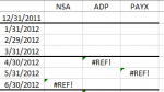
Columns B, E, and G have dates and Columns C, D, F, and H have data that i have input

I would like to transfer data to Column K, L, and M if the dates from Column J match the dates in Column B, E, or G and the headings from row with labels (circled in red) match.

Thank you very much in advance for your help.

 

[AlanY]

try this, you may need to unmerge the column header cells to work

Book1
	A	B	C	D	E	F	G	H	I	J	K	L	M
1				NSA		ADP		PAYX			NSA	ADP	PAYX
2		31/08/2020		1%	31/08/2020	2%	31/08/2020	0.5%		31/08/2020	1%	2%	0.5%
3		24/08/2020		2%	22/08/2020	4%	24/08/2020	1.0%		24/08/2020
4		17/08/2020		4%	17/08/2020	8%	17/08/2020	2.0%		17/08/2020	4%	8%	2.0%
5		10/08/2020		8%	10/08/2020	16%	11/08/2020	4.0%		10/08/2020
6		03/08/2020		16%	01/08/2020	32%	03/08/2020	8.0%		03/08/2020
7		27/07/2020		32%	27/07/2020	64%	27/07/2020	16.0%		27/07/2020	32%	64%	16.0%
Sheet5

Cell Formulas
Range	Formula
K2:M7	K2	=IF(AND($J2=$B2,$J2=$E2,$J2=$G2),INDEX($A2:$I2,MATCH(K$1,$A$1:$I$1,0)),"")

 

[whynot]

Thank you very much for the reply.

It did not work - I believe its because I need to lookup all the dates in column B, E, and G and try to match with column J. For example, the date in J2 would match with the date in B5 and the data i need is in d2. I hope that makes sense.

 

[AlanY]

ok, how about?

Book1
	A	B	C	D	E	F	G	H	I	J	K	L	M
1				NSA		ADP		PAYX			NSA	ADP	PAYX
2		23/08/2020		1%	21/08/2020	2%	31/08/2020	1%		31/08/2020	8%	4%	1%
3		24/08/2020		2%	31/08/2020	4%	24/08/2020	1%
4		17/08/2020		4%	17/08/2020	8%	17/08/2020	2%
5		31/08/2020		8%	31/07/2020	16%	11/08/2020	4%
6		03/08/2020		16%	01/08/2020	32%	03/08/2020	8%
7		27/07/2020		32%	27/07/2020	64%	27/07/2020	16%
Sheet7

Cell Formulas
Range	Formula
K2	K2	=INDEX(D:D,MATCH($J$2,B:B,0))
L2	L2	=INDEX(F:F,MATCH($J$2,E:E,0))
M2	M2	=INDEX(H:H,MATCH($J$2,G:G,0))

 

[whynot]

Thank you so much!!! That works.

If i am not bothering - a "#NA" is displayed in columns where there are no matches. Is there a way to write the formula so the column remains blank - does not show anything.

Thank you.

 

[AlanY]

you're welcome, you can use a iferror() function like this;

=iferror(INDEX(D:D,MATCH($J$2,B:B,0)),"")

 

[whynot]

That works!!!

Thank you very much!!!

I really appreciate the help.

Have a great day!!!

 

[ER_Neha]

Hello Here is another formula that you can use.

Book1
	A	B	C	D	E	F	G	H	I	J	K	L	M
1	Quarter	Month	SA	NSA		ADP		PAYX			NSA	ADP	PAYX
2		31-03-2011	7	8	30-04-2011	7	31-05-2011	2		31-12-2011	2
3		30-06-2011	0	0	31-07-2011	5	31-08-2011	4		31-01-2012		5
4		30-09-2011	2	2	31-10-2011	7	30-11-2011	3		29-02-2012			4
5		31-12-2011	2	2	31-01-2012	5	29-02-2012	4		31-03-2012
6										30-04-2012
7										31-05-2012
8										30-06-2012
Sheet1

Cell Formulas
Range	Formula
K2:K8	K2	=XLOOKUP(J2,$B$2:$B$5,$D$2:$D$5,"")
L2:L8	L2	=XLOOKUP(J2,$E$2:$E$5,$F$2:$F$5,"")
M2:M8	M2	=XLOOKUP(J2,$G$2:$G$5,$H$2:$H$5,"")

 

[whynot]

thank you for the help!! I really appreciate it!!!