Match and sort different sized data sets

[Hammer123]

Hi,

I have a query regarding matching and sorting different sized data sheets. There was a question regarding this a while ago and a VBA solution posted - however I cant seem to figure out how to amend it to suit the worksheet I have. Really hoping someone can help me out - hopefully I have explained it well enough and it makes sense.

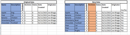
In short I have some original data (columns A to G). I then have some new data (columns I to P).

I want to run a VBA code to sort the columns I & J (including carrying the data from columns K to P) to match up with columns A & B. Data in A&B and I&J needs to match otherwise if it doesn't it would move it to a empty cell at the bottom of the last row.

If there is the same name and description listed twice in columns I & J, it would then create a new row across the workbook, copy the data in the original, intent it and colour it red to show its a duplicate.

Once sorted, I then want to run some conditional formatting to highlight if the cells in column L matches the cells in column E. If it does and it is the same then it highlight the cell in L green. If not it highlights the cell in column L red.

E.g. something like this.....

From this

To this

If anyone can help me or suggest a better way to do it, would be much appreciated. Hoping I have explained myself enough. Newbie here!

 

[Eric W]

Welcome to the MrExcel forum!

Starting with this (Conditional Formatting included):

Book2
	A	B	C	D	E	F	G	H	I	J	K	L	M	N	O	P
1
2	Name	Description	Included	Revision	Status	Date Created	Originator		Name	Description	Included	Revision	Status	Date Created	Originator	Yes/no
3	Apple	Dog	X	1	4	1/11/2023	Joe Bloggs		Chocolate	Football	x	4	4	1/11/2023	Joe Bloggs	Yes
4	Pear	Cat	X	2	4	1/11/2023	Joe Bloggs		Apple	Dog	x	3	4	1/11/2023	Joe Bloggs	Yes
5	Banana	Chicken	X	3	4	1/11/2023	Joe Bloggs		Banana	Chicken	x	2	4	1/11/2023	Joe Bloggs	Yes
6	Strawberry	Boat	X	4	4	1/11/2023	Joe Bloggs		Strawberry	Boat	x	5	4	1/11/2023	Joe Bloggs	Yes
7	Chocolate	Football	X	1	4	1/11/2023	Joe Bloggs		Pear	Cat	x	1	4	1/11/2023	Joe Bloggs	Yes
8									Pear	Cat	x	2	4	1/11/2023	Joe Bloggs	Yes
9									Banana	Chicken	x	3	4	1/11/2023	Joe Bloggs	Yes
10									Fox	Rugby	x	7	4	1/11/2023	Joe Bloggs	Yes
11
Sheet6

Cells with Conditional Formatting
Cell	Condition		Cell Format	Stop If True
L3:L20	Expression	=AND(A3=I3,D3=L3,L3<>"")	text	NO
A4:B20	Expression	=A4=A3	text	NO
L3:L20	Expression	=L3<>""	text	NO
A3:B20,I3:J20	Expression	=A3<>""	text	NO
A2:G20,I2:P20	Expression	=A2<>""	text	NO

You can run this macro:

Sub SortAndCompare()
Dim lr1 As Long, lr2 As Long, r As Long, r1 As Long, r2 As Long, c As Long
Dim dat As Variant, datn As Variant, dat2 As Variant

    lr1 = Cells(Rows.Count, "A").End(xlUp).Row
    lr2 = Cells(Rows.Count, "I").End(xlUp).Row
    
    Columns("Q:Q").Insert shift:=xlToRight
    Range("Q3:Q" & lr2).Formula = "=IFERROR(MATCH(I3,$A$3:$A$" & lr1 & ",0),9^9)"
    Range("Q3:Q" & lr2).Value = Range("Q3:Q" & lr2).Value
    With ActiveSheet.Sort
        .SortFields.Clear
        .SortFields.Add2 Key:=Range("Q3:Q" & lr2), Order:=xlAscending
        .SetRange Range("I2:Q" & lr2)
        .Header = xlYes
        .Apply
    End With
    
    Columns("Q:Q").Delete shift:=xlToLeft
    
    dat = Range("A4:G" & lr2).Value
    datn = dat
    dat2 = Range("I4:P" & lr2).Value
    
    r1 = 1
    
    For r2 = 1 To UBound(dat2)
        If dat(r1, 1) <> dat2(r2, 1) Then r1 = r1 + 1
        For c = 1 To 7
            datn(r2, c) = dat(r1, c)
        Next c
    Next r2
    
    Range("A4").Resize(UBound(dat2), 7).Value = datn
            
End Sub

And you'll end up with this:

Book2
	A	B	C	D	E	F	G	H	I	J	K	L	M	N	O	P
1
2	Name	Description	Included	Revision	Status	Date Created	Originator		Name	Description	Included	Revision	Status	Date Created	Originator	Yes/no
3	Apple	Dog	X	1	4	1/11/2023	Joe Bloggs		Apple	Dog	x	3	4	1/11/2023	Joe Bloggs	Yes
4	Pear	Cat	X	2	4	1/11/2023	Joe Bloggs		Pear	Cat	x	1	4	1/11/2023	Joe Bloggs	Yes
5	Pear	Cat	X	2	4	1/11/2023	Joe Bloggs		Pear	Cat	x	2	4	1/11/2023	Joe Bloggs	Yes
6	Banana	Chicken	X	3	4	1/11/2023	Joe Bloggs		Banana	Chicken	x	2	4	1/11/2023	Joe Bloggs	Yes
7	Banana	Chicken	X	3	4	1/11/2023	Joe Bloggs		Banana	Chicken	x	3	4	1/11/2023	Joe Bloggs	Yes
8	Strawberry	Boat	X	4	4	1/11/2023	Joe Bloggs		Strawberry	Boat	x	5	4	1/11/2023	Joe Bloggs	Yes
9	Chocolate	Football	X	1	4	1/11/2023	Joe Bloggs		Chocolate	Football	x	4	4	1/11/2023	Joe Bloggs	Yes
10									Fox	Rugby	x	7	4	1/11/2023	Joe Bloggs	Yes
11
Sheet6

Cells with Conditional Formatting
Cell	Condition		Cell Format	Stop If True
L3:L20	Expression	=AND(A3=I3,D3=L3,L3<>"")	text	NO
A4:B20	Expression	=A4=A3	text	NO
L3:L20	Expression	=L3<>""	text	NO
A3:B20,I3:J20	Expression	=A3<>""	text	NO
A2:G20,I2:P20	Expression	=A2<>""	text	NO

Try it on a copy of your workbook first.

 

[Hammer123]

Hi Eric,

Many thanks for your help, it is very much appreciated - I have run it on my workbook and this is what I get. Have included the Conditional Format tab as well so you can see if I have made any errors.

Looks like it sorts the data on the right table, but then doesn't align/move it to the rows on the left, nor does it create an additional line.

Can you help? Thank you in advance.

 

[Eric W]

Hmm, I'm puzzled. I can't understand why the first part of the macro, that sorts the right table, works, but the second half that adjusts the left table doesn't. There might be something subtle going on that I'm missing. Can you install the xl2bb add-in, and then provide a mini-sheet with your initial tables? Similar to how I did in post 2? There's a link in the reply box, or my signature. It's easy to install and use.

One thing I noticed is that the first of your Conditional Formatting rules is missing a format. It should have a full outside border. This was done to make the grid for the table on the left expand as the new rows were added. This can actually be done in the macro (like some of the other CF rules), but it was easier this way. But it could depend on the way your initial table is actually generated.

 

[Hammer123]

Test.xlsm
	A	B	C	D	E	F	G	H	I	J	K	L	M	N	O	P
2	Original Data								New Data
3	Name	Description	Included	Revision	Status	Date Created	Originator		Name	Description	Included	Revision	Status	Date Created	Originator	Yes/No
4	Apple	Dog	X	1	4	01/11/2023	Joe Bloggs		Apple	Dog	X	3	4	01/11/2023	Joe Bloggs	Yes
5	Pear	Cat	X	2	4	01/11/2023	Joe Bloggs		Banana	Chicken	X	2	4	01/11/2023	Joe Bloggs	Yes
6	Banana	Chicken	X	3	4	01/11/2023	Joe Bloggs		Banana	Chicken	X	3	4	01/11/2023	Joe Bloggs	Yes
7	Strawberry	Boat	X	4	4	01/11/2023	Joe Bloggs		Strawberry	Boat	X	5	4	01/11/2023	Joe Bloggs	Yes
8	Chocolate	Football	X	1	4	01/11/2023	Joe Bloggs		Chocolate	Football	X	4	4	01/11/2023	Joe Bloggs	Yes
9									Pear	Cat	X	1	4	01/11/2023	Joe Bloggs	Yes
10									Pear	Cat	X	2	4	01/11/2023	Joe Bloggs	Yes
11									Fox	Rugby	X	7	4	01/11/2023	Joe Bloggs	Yes
12
Sheet1

Cells with Conditional Formatting
Cell	Condition		Cell Format	Stop If True
A2:G20,I2:P20	Expression	=A2<>""	text	NO
A3:B20,I3:J20	Expression	=A3<>""	text	NO
L3:L20	Expression	=L3<>""	text	NO
A4:B20	Expression	=A4=A3	text	NO
L3:L20	Expression	=" =AND(A3=I3,D3=L3,L3<>"""")"	text	NO

 

[Eric W]

OK, I found 2 issues. First, I was inconsistent with the top row of the data. Your original post shows the tables starting on row 3, my first macro requires it to start on row 2. To handle that, I changed the macro so that the addresses of the tables are entered at the top. You can see the "Set OrgData = ", and "Set NewData = " lines are, set that to the appropriate ranges. The rest of the macro will refer to those ranges.

Second, when is a pear not a pear? When the pear in the new data table has a space on the end. Because of that, it wasn't matching the pear in the original data table, so it didn't sort in the proper order.

Here's the updated macro:

Sub SortAndCompare()
Dim nc As Long, r As Long, r1 As Long, r2 As Long, c As Long
Dim dat As Variant, datn As Variant, dat2 As Variant
Dim OrgData As Range, NewData As Range

    Set OrgData = Range("A3:G8")
    Set NewData = Range("I3:P11")
    
    nc = NewData.Column + NewData.Columns.Count
    Columns(nc).Insert
    Cells(NewData.Row, nc).Resize(NewData.Rows.Count).Formula = _
          "=IFERROR(MATCH(" & NewData(1, 1).Address(0, 0) & "," & _
            OrgData.Resize(, 1).Address & ",0),9^9)"
            
    With ActiveSheet.Sort
        .SortFields.Clear
        .SortFields.Add2 Key:=Cells(NewData.Row + 1, nc), Order:=xlAscending
        .SetRange NewData.Resize(, NewData.Columns.Count + 1)
        .Header = xlYes
        .Apply
    End With
    
    Columns(nc).Delete Shift:=xlToLeft
    
    dat = OrgData.Resize(NewData.Rows.Count).Value
    datn = dat
    dat2 = NewData.Value
    
    r1 = 2
    
    For r2 = 2 To UBound(dat2)
        If dat(r1, 1) <> dat2(r2, 1) Then r1 = r1 + 1
        For c = 1 To OrgData.Columns.Count
            datn(r2, c) = dat(r1, c)
        Next c
    Next r2
    
    OrgData.Resize(UBound(dat2)).Value = datn
            
End Sub

Try this version, and make sure that the names in both tables match. Let us know how it works!

 

[Hammer123]

Hi Eric,

Many thanks for the prompt reply, when I ran it, nothing seemed to change.

I also tried it on a completely new workbook to see if I had done something wrong but ended up with the same result.

 

[Eric W]

I'm not sure how to help you at this point. I painstakingly recreated your sheet from post 5 from scratch, including all data and CF rules. I removed the space from the end of "pear". I then ran the macro from post 6, updating the ranges appropriately, and recreated the results from post 2. There were a few minor issues with the CF rules, but the left table was created correctly. All I can think is there's some subtle difference in our sheets, but I certainly can't see it.

 

[Hammer123]

thank you Eric - I really appreciate the time and effort you have gone in to.

Is there a way to send the file you managed to do it in?