Index Match

Todd Kolar

New Member
Joined
Feb 7, 2024
Messages
10
Office Version
  1. 2016
Platform
  1. Windows
I can never figure out how to use index with match as I have researched how the syntax works.
I guess my brain cannot comprehend it or something.
So basically, I need to match some data together that have the same information.
I have attached 2 screenshots because I cannot download the other option (our IT is super strict).
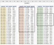
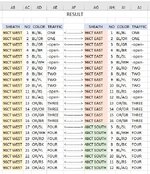
The main identical information is in the "Traffic" columns.
So it needs to pull the data if they match.
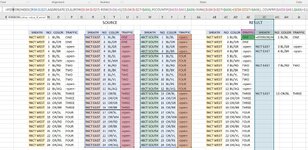
Columns M through Z show how the data will display and columns AB though AJ is how I need it to display.
Columns M though P in the noted source area will always be a constant where columns R though Z will differ.
So in the noted result area, columns AB though AE will basically be a copy, but columns AG though AJ will reflect what matches.
I hope I explained this well in addition to the screenshot with notes.
Y'all will be my heroes if you can offer any assistance and I thank all in advance for reading my "novel" of a post.
 

Attachments

  • Excel Help3.JPG
    Excel Help3.JPG
    151.5 KB · Views: 18
  • Excel Help4.JPG
    Excel Help4.JPG
    110.8 KB · Views: 18

Excel Facts

Excel motto
Not everything I do at work revolves around Excel. Only the fun parts.
Just to confirm...this uses an approach that should work in Excel 2016 (you are not using Excel 365/2021?):
MrExcel_20240213.xlsx
MNOPQRSTUVWXYZAAABACADAEAFAGAHAI
1SOURCERESULTS
2
3SHEATHNOCOLORTRAFFICSHEATHNOCOLORTRAFFICCOLORNOCOLORTRAFFICSHEATHNOCOLORTRAFFICSHEATHNOCOLORTRAFFIC
496CT WEST1BL/BLONE96CT EAST1BL/BLONE48CT SOUTH1BL/BL-open-96CT WEST1BL/BLONE96CT EAST1BL/BLONE
596CT WEST2BL/ORONE96CT EAST2BL/ORONE48CT SOUTH2BL/OR-open-96CT WEST2BL/ORONE96CT EAST2BL/ORONE
696CT WEST3BL/GR-open-96CT EAST3BL/GR-open-48CT SOUTH3BL/GR-open-96CT WEST3BL/GR-open-96CT EAST3BL/GR-open-
796CT WEST4BL/BR-open-96CT EAST4BL/BR-open-48CT SOUTH4BL/BR-open-96CT WEST4BL/BR-open-96CT EAST4BL/BR-open-
896CT WEST5BL/SL-open-96CT EAST5BL/SL-open-48CT SOUTH5BL/SLFOUR96CT WEST5BL/SL-open-96CT EAST5BL/SL-open-
996CT WEST6BL/WH-open-96CT EAST6BL/WH-open-48CT SOUTH6BL/WHFOUR96CT WEST6BL/WH-open-96CT EAST6BL/WH-open-
1096CT WEST7BL/RDTWO96CT EAST7BL/RDTWO48CT SOUTH7BL/RDFOUR96CT WEST7BL/RDTWO96CT EAST7BL/RDTWO
1196CT WEST8BL/BKTWO96CT EAST 8BL/BKTWO48CT SOUTH8BL/BKFOUR96CT WEST8BL/BKTWO96CT EAST 8BL/BKTWO
1296CT WEST9BL/YLTWO96CT EAST9BL/YLTWO48CT SOUTH9BL/YLFOUR96CT WEST9BL/YLTWO96CT EAST9BL/YLTWO
1396CT WEST10BL/VLTWO96CT EAST10BL/VLTWO48CT SOUTH10BL/VLFOUR96CT WEST10BL/VLTWO96CT EAST10BL/VLTWO
1496CT WEST11BL/RS-open-96CT EAST11BL/RS-open-48CT SOUTH11BL/RSFOUR96CT WEST11BL/RS-open-96CT EAST11BL/RS-open-
1596CT WEST12BL/AQ-open-96CT EAST12BL/AQ-open-48CT SOUTH12BL/AQFOUR96CT WEST12BL/AQ-open-96CT EAST12BL/AQ-open-
1696CT WEST13OR/BLTHREE96CT EAST13OR/BLTHREE48CT SOUTH13OR/BL-open-96CT WEST13OR/BLTHREE96CT EAST13OR/BLTHREE
1796CT WEST14OR/ORTHREE96CT EAST14OR/ORTHREE48CT SOUTH14OR/OR-open-96CT WEST14OR/ORTHREE96CT EAST14OR/ORTHREE
1896CT WEST15OR/GRTHREE96CT EAST15OR/GRTHREE48CT SOUTH15OR/GR-open-96CT WEST15OR/GRTHREE96CT EAST15OR/GRTHREE
1996CT WEST16OR/BRTHREE96CT EAST16OR/BRTHREE48CT SOUTH16OR/BR-open-96CT WEST16OR/BRTHREE96CT EAST16OR/BRTHREE
2096CT WEST17OR/SLFOUR96CT EAST17OR/SL-open-48CT SOUTH17OR/SL-open-96CT WEST17OR/SLFOUR48CT SOUTH5BL/SLFOUR
2196CT WEST18OR/WHFOUR96CT EAST18OR/WH-open-48CT SOUTH18OR/WH-open-96CT WEST18OR/WHFOUR48CT SOUTH6BL/WHFOUR
2296CT WEST19OR/RDFOUR96CT EAST19OR/RD-open-48CT SOUTH19OR/RD-open-96CT WEST19OR/RDFOUR48CT SOUTH7BL/RDFOUR
2396CT WEST20OR/BKFOUR96CT EAST20OR/BK-open-48CT SOUTH20OR/BK-open-96CT WEST20OR/BKFOUR48CT SOUTH8BL/BKFOUR
2496CT WEST21OR/YLFOUR96CT EAST21OR/YL-open-48CT SOUTH21OR/YL-open-96CT WEST21OR/YLFOUR48CT SOUTH9BL/YLFOUR
2596CT WEST22OR/VLFOUR96CT EAST22OR/VL-open-48CT SOUTH22OR/VL-open-96CT WEST22OR/VLFOUR48CT SOUTH10BL/VLFOUR
2696CT WEST23OR/RSFOUR96CT EAST23OR/RS-open-48CT SOUTH23OR/RS-open-96CT WEST23OR/RSFOUR48CT SOUTH11BL/RSFOUR
2796CT WEST24OR/AQFOUR96CT EAST24OR/AQ-open-48CT SOUTH24OR/AQ-open-96CT WEST24OR/AQFOUR48CT SOUTH12BL/AQFOUR
Sheet1
Cell Formulas
RangeFormula
AB4:AE27AB4=M4:P4
AF4:AI27AF4=IFERROR( INDEX($R$4:$U$27, AGGREGATE(15,6,(ROW($U$4:$U$27)-ROW($U$4)+1)/($U$4:$U$27=$AE4), IF(COUNTIF($AE$3:$AE3,$AE4)<SUM(($U$4:$U$27=$AE4)+($Z$4:$Z$27=$AE4)), COUNTIF($AE$3:$AE3,$AE4)+1)),), IFERROR( INDEX($W$4:$Z$27, AGGREGATE(15,6,(ROW($Z$4:$Z$27)-ROW($Z$4)+1)/($Z$4:$Z$27=$AE4), IF(COUNTIF($AE$3:$AE3,$AE4)<SUM(($U$4:$U$27=$AE4)+($Z$4:$Z$27=$AE4)), COUNTIF($AE$3:$AE3,$AE4)+1)),), ""))
Dynamic array formulas.
 
Upvote 0
Yes I am using Excel 2016, however, I copied and pasted the formula exactly how you have it and unfortunately it did not work.
I then tried the array function (ctl+shift+enter) thinking it was an array formula and nothing happened there either.
I must be doing something wrong because it works for you.
 
Upvote 0
I doubt that you are doing anything wrong...rather I haven't adjusted to formula to work correctly with Excel 2016. This version is even messier, but it should work when dragged throughout:
MrExcel_20240213.xlsx
MNOPQRSTUVWXYZAAABACADAEAFAGAHAI
1SOURCERESULTS
2
3SHEATHNOCOLORTRAFFICSHEATHNOCOLORTRAFFICCOLORNOCOLORTRAFFICSHEATHNOCOLORTRAFFICSHEATHNOCOLORTRAFFIC
496CT WEST1BL/BLONE96CT EAST1BL/BLONE48CT SOUTH1BL/BL-open-96CT WEST1BL/BLONE96CT EAST1BL/BLONE
596CT WEST2BL/ORONE96CT EAST2BL/ORONE48CT SOUTH2BL/OR-open-96CT WEST2BL/ORONE96CT EAST2BL/ORONE
696CT WEST3BL/GR-open-96CT EAST3BL/GR-open-48CT SOUTH3BL/GR-open-96CT WEST3BL/GR-open-96CT EAST3BL/GR-open-
796CT WEST4BL/BR-open-96CT EAST4BL/BR-open-48CT SOUTH4BL/BR-open-96CT WEST4BL/BR-open-96CT EAST4BL/BR-open-
896CT WEST5BL/SL-open-96CT EAST5BL/SL-open-48CT SOUTH5BL/SLFOUR96CT WEST5BL/SL-open-96CT EAST5BL/SL-open-
996CT WEST6BL/WH-open-96CT EAST6BL/WH-open-48CT SOUTH6BL/WHFOUR96CT WEST6BL/WH-open-96CT EAST6BL/WH-open-
1096CT WEST7BL/RDTWO96CT EAST7BL/RDTWO48CT SOUTH7BL/RDFOUR96CT WEST7BL/RDTWO96CT EAST7BL/RDTWO
1196CT WEST8BL/BKTWO96CT EAST 8BL/BKTWO48CT SOUTH8BL/BKFOUR96CT WEST8BL/BKTWO96CT EAST 8BL/BKTWO
1296CT WEST9BL/YLTWO96CT EAST9BL/YLTWO48CT SOUTH9BL/YLFOUR96CT WEST9BL/YLTWO96CT EAST9BL/YLTWO
1396CT WEST10BL/VLTWO96CT EAST10BL/VLTWO48CT SOUTH10BL/VLFOUR96CT WEST10BL/VLTWO96CT EAST10BL/VLTWO
Sheet1
Cell Formulas
RangeFormula
AB4:AE13AB4=INDEX($M4:$P4,1,COLUMNS($AB:AB))
AF4:AI13AF4=IFERROR( INDEX($R$4:$U$27, AGGREGATE(15,6,(ROW($U$4:$U$27)-ROW($U$4)+1)/($U$4:$U$27=$AE4), IF(COUNTIF($AE$3:$AE3,$AE4)<SUM(($U$4:$U$27=$AE4)+($Z$4:$Z$27=$AE4)), COUNTIF($AE$3:$AE3,$AE4)+1)),COLUMNS($AF:AF)), IFERROR( INDEX($W$4:$Z$27, AGGREGATE(15,6,(ROW($Z$4:$Z$27)-ROW($Z$4)+1)/($Z$4:$Z$27=$AE4), IF(COUNTIF($AE$3:$AE3,$AE4)<SUM(($U$4:$U$27=$AE4)+($Z$4:$Z$27=$AE4)), COUNTIF($AE$3:$AE3,$AE4)+1)),COLUMNS($AF:AF)), ""))
 
Upvote 0
It populated only a few cells so I'm not sure why it isn't working on my end.
It works perfectly on yours.
I'm baffled.
My Excel is cursed... lololol
 

Attachments

  • Excel Help5.JPG
    Excel Help5.JPG
    247.8 KB · Views: 5
Upvote 0
Could you copy the formula in the first row, first cell…AF4, I think, and paste it directly into a post here. You can wrap it inside the code brackets provided by the “fx xls” button in the posting window for better formatting.
 
Upvote 0
Excel Formula:
=IFERROR(INDEX($R$4:$U$27,AGGREGATE(15,6,(ROW($U$4:$U$27)-ROW($U$4)+1)/($U$4:$U$27=$AE4),IF(COUNTIF($AE$3:$AE3,$AE4)<SUM(($U$4:$U$27=$AE4)+($Z$4:$Z$27=$AE4)), COUNTIF($AE$3:$AE3,$AE4)+1)),COLUMNS($AF:AF)),IFERROR(INDEX($W$4:$Z$27, AGGREGATE(15,6,(ROW($Z$4:$Z$27)-ROW($Z$4)+1)/($Z$4:$Z$27=$AE4),IF(COUNTIF($AE$3:$AE3,$AE4)<SUM(($U$4:$U$27=$AE4)+($Z$4:$Z$27=$AE4)), COUNTIF($AE$3:$AE3,$AE4)+1)),COLUMNS($AF:AF)), ""))
Excel Formula:
 
Upvote 0
Let's run a quick check on your source data...enter this formula and copy down to get a count of the number of matching items. I'm wondering if a hidden character or space might be present.
MrExcel_20240213.xlsx
KLMNOP
1SOURCE
2
3SHEATHNOCOLORTRAFFIC
4296CT WEST1BL/BLONE
5296CT WEST2BL/ORONE
6696CT WEST3BL/GR-open-
7696CT WEST4BL/BR-open-
8696CT WEST5BL/SL-open-
9696CT WEST6BL/WH-open-
10496CT WEST7BL/RDTWO
11496CT WEST8BL/BKTWO
12496CT WEST9BL/YLTWO
13496CT WEST10BL/VLTWO
14696CT WEST11BL/RS-open-
15696CT WEST12BL/AQ-open-
16496CT WEST13OR/BLTHREE
17496CT WEST14OR/ORTHREE
18496CT WEST15OR/GRTHREE
19496CT WEST16OR/BRTHREE
20896CT WEST17OR/SLFOUR
21896CT WEST18OR/WHFOUR
22896CT WEST19OR/RDFOUR
23896CT WEST20OR/BKFOUR
24896CT WEST21OR/YLFOUR
25896CT WEST22OR/VLFOUR
26896CT WEST23OR/RSFOUR
27896CT WEST24OR/AQFOUR
Sheet1
Cell Formulas
RangeFormula
K4:K27K4=COUNTIF($P$4:$P$27,P4)

Side note: when you click on the "fx xls" button, a set of start and end "code=xls" markers will be inserted...they are each surrounded by square brackets in your post...you paste your formula in between the two sets of markers.
 
Last edited:
Upvote 0
Let's run a quick check on your source data...enter this formula and copy down to get a count of the number of matching items. I'm wondering if a hidden character or space might be present.
MrExcel_20240213.xlsx
KLMNOP
1SOURCE
2
3SHEATHNOCOLORTRAFFIC
4296CT WEST1BL/BLONE
5296CT WEST2BL/ORONE
6696CT WEST3BL/GR-open-
7696CT WEST4BL/BR-open-
8696CT WEST5BL/SL-open-
9696CT WEST6BL/WH-open-
10496CT WEST7BL/RDTWO
11496CT WEST8BL/BKTWO
12496CT WEST9BL/YLTWO
13496CT WEST10BL/VLTWO
14696CT WEST11BL/RS-open-
15696CT WEST12BL/AQ-open-
16496CT WEST13OR/BLTHREE
17496CT WEST14OR/ORTHREE
18496CT WEST15OR/GRTHREE
19496CT WEST16OR/BRTHREE
20896CT WEST17OR/SLFOUR
21896CT WEST18OR/WHFOUR
22896CT WEST19OR/RDFOUR
23896CT WEST20OR/BKFOUR
24896CT WEST21OR/YLFOUR
25896CT WEST22OR/VLFOUR
26896CT WEST23OR/RSFOUR
27896CT WEST24OR/AQFOUR
Sheet1
Cell Formulas
RangeFormula
K4:K27K4=COUNTIF($P$4:$P$27,P4)

Side note: when you click on the "fx xls" button, a set of start and end "code=xls" markers will be inserted...they are each surrounded by square brackets in your post...you paste your formula in between the two sets of markers.
I performed the tasked you asked and got the same results.
Looks like no spaces or hidden characters.
It should work on my end so I'm so confused why it isn't.
 
Upvote 0
Okay...thanks. Give this version a try. I want to avoid the array produced by making a logical test of a range being equal to a specific value, so I've changed the SUM portion of the formula.
Cell Formulas
RangeFormula
AB4:AE11AB4=INDEX($M4:$P4,1,COLUMNS($AB:AB))
AF4:AI11AF4=IFERROR( INDEX($R$4:$U$27, AGGREGATE(15,6,(ROW($U$4:$U$27)-ROW($U$4)+1)/($U$4:$U$27=$AE4), IF(COUNTIF($AE$3:$AE3,$AE4)<(COUNTIF($U$4:$U$27,$AE4)+COUNTIF($Z$4:$Z$27,$AE4)), COUNTIF($AE$3:$AE3,$AE4)+1)),COLUMNS($AF:AF)), IFERROR( INDEX($W$4:$Z$27, AGGREGATE(15,6,(ROW($Z$4:$Z$27)-ROW($Z$4)+1)/($Z$4:$Z$27=$AE4), IF(COUNTIF($AE$3:$AE3,$AE4)<(COUNTIF($U$4:$U$27,$AE4)+COUNTIF($Z$4:$Z$27,$AE4)), COUNTIF($AE$3:$AE3,$AE4)+1)),COLUMNS($AF:AF)), ""))
 
Upvote 0

Forum statistics

Threads
1,215,069
Messages
6,122,959
Members
449,096
Latest member
Anshu121

We've detected that you are using an adblocker.

We have a great community of people providing Excel help here, but the hosting costs are enormous. You can help keep this site running by allowing ads on MrExcel.com.
Allow Ads at MrExcel

Which adblocker are you using?

Disable AdBlock

Follow these easy steps to disable AdBlock

1)Click on the icon in the browser’s toolbar.
2)Click on the icon in the browser’s toolbar.
2)Click on the "Pause on this site" option.
Go back

Disable AdBlock Plus

Follow these easy steps to disable AdBlock Plus

1)Click on the icon in the browser’s toolbar.
2)Click on the toggle to disable it for "mrexcel.com".
Go back

Disable uBlock Origin

Follow these easy steps to disable uBlock Origin

1)Click on the icon in the browser’s toolbar.
2)Click on the "Power" button.
3)Click on the "Refresh" button.
Go back

Disable uBlock

Follow these easy steps to disable uBlock

1)Click on the icon in the browser’s toolbar.
2)Click on the "Power" button.
3)Click on the "Refresh" button.
Go back
Back
Top