Index Match

Todd Kolar

New Member
Joined
Feb 7, 2024
Messages
10
Office Version
  1. 2016
Platform
  1. Windows
I can never figure out how to use index with match as I have researched how the syntax works.
I guess my brain cannot comprehend it or something.
So basically, I need to match some data together that have the same information.
I have attached 2 screenshots because I cannot download the other option (our IT is super strict).
The main identical information is in the "Traffic" columns.
So it needs to pull the data if they match.
Columns M through Z show how the data will display and columns AB though AJ is how I need it to display.
Columns M though P in the noted source area will always be a constant where columns R though Z will differ.
So in the noted result area, columns AB though AE will basically be a copy, but columns AG though AJ will reflect what matches.
I hope I explained this well in addition to the screenshot with notes.
Y'all will be my heroes if you can offer any assistance and I thank all in advance for reading my "novel" of a post.
 

Attachments

  • Excel Help3.JPG
    Excel Help3.JPG
    151.5 KB · Views: 18
  • Excel Help4.JPG
    Excel Help4.JPG
    110.8 KB · Views: 18
That worked perfectly!
Now, how do I expand it to grab more columns?
I tried to examine your formula, but I don't have the brain power to make it work.
Attached is a pic of the other columns I'd like to include up to column AV.
The cell that has your formula is BC8.
And most importantly thank you very much for your help on this!!!!!
If you can get it to work for the additional columns, you'll be my hero!
 

Attachments

  • Excel Help6.JPG
    Excel Help6.JPG
    231 KB · Views: 6
Upvote 0

Excel Facts

Why are there 1,048,576 rows in Excel?
The Excel team increased the size of the grid in 2007. There are 2^20 rows and 2^14 columns for a total of 17 billion cells.
Good news...that it worked for you. Now for the bad news...I discovered a vulnerability with the formula: when attempting to keep your tables separate, and matching is done table-by-table moving from left to right, it becomes necessary to know how many matches have been made for a given "Traffic" code. This is due to the need to specify within AGGREGATE which of potentially multiple Traffic matches within a column need to be delivered by the formula, and we cannot simply count the way I had anticipated because prior matches exist in multiple other ranges. So the formula becomes messy quickly, as the component of the formula that deals with each table requires a sequential count of previously processed tables...so there is a lot of redundancy and many range references to manage. If you had only a couple of tables, this is probably okay to deal with, but after about three tables, I wouldn't recommend this approach. It will work, but it would be very difficult to maintain and edit reliably. Here is what it looks like for a Source table at left and 6 Group tables structured similarly to your example. The results are in AZ:BA for the Source table repeat, and BC:BF for the sequential matches throughout. Due to posting size limits, I'm not sure I can post the entire sheet, so I may need to do it piecemeal:
MrExcel_20240213b.xlsx
MNOPQRSTUVWXYZAAABACADAEAFAGAHAIAJAKALAMANAOAPAQARASATAUAV
1SOURCEGROUP 1GROUP 2GROUP 3GROUP 4GROUP 5GROUP 6
2
3SHEATHNOCOLORTRAFFICSHEATHNOCOLORTRAFFICCOLORNOCOLORTRAFFIC
496CT WEST1BL/BLONE96CT EAST1BL/BL-open-48CT SOUTH1BL/BL-open-
596CT WEST2BL/ORONE96CT EAST2BL/ORONE48CT SOUTH2BL/OR-open-
696CT WEST3BL/GR-open-96CT EAST3BL/GR-open-48CT SOUTH3BL/GRTWO
796CT WEST4BL/BRTWO96CT EAST4BL/BR-open-48CT SOUTH4BL/BR-open-COLORNOCOLORTRAFFICCOLORNOCOLORTRAFFICCOLORNOCOLORTRAFFICCOLORNOCOLORTRAFFIC
896CT WEST5BL/SLTWO96CT EAST5BL/SL-open-48CT SOUTH5BL/SLFOUR48CT SOUTH1BL/BL-open-48CT SOUTH1BL/BL-open-48CT SOUTH1BL/BL-open-48CT SOUTH1BL/BL-open-
996CT WEST6BL/WH-open-96CT EAST6BL/WH-open-48CT SOUTH6BL/WH-open-48CT SOUTH2BL/ORONE48CT SOUTH2BL/OR-open-48CT SOUTH2BL/OR-open-48CT SOUTH2BL/OR-open-
1096CT WEST7BL/RDTWO96CT EAST7BL/RD-open-48CT SOUTH7BL/RDFOUR48CT SOUTH3BL/GR-open-48CT SOUTH3BL/GR-open-48CT SOUTH3BL/GRTWO48CT SOUTH3BL/GR-open-
1196CT WEST8BL/BKTWO96CT EAST 8BL/BKTWO48CT SOUTH8BL/BK-open-48CT SOUTH4BL/BR-open-48CT SOUTH4BL/BR-open-48CT SOUTH4BL/BR-open-48CT SOUTH4BL/BR-open-
1296CT WEST9BL/YLTWO96CT EAST9BL/YL-open-48CT SOUTH9BL/YLFOUR48CT SOUTH5BL/SL-open-48CT SOUTH5BL/SLFOUR48CT SOUTH5BL/SL-open-48CT SOUTH5BL/SLFOUR
1396CT WEST10BL/VLTWO96CT EAST10BL/VLTWO48CT SOUTH10BL/VL-open-48CT SOUTH6BL/WH-open-48CT SOUTH6BL/WH-open-48CT SOUTH6BL/WHTHREE48CT SOUTH6BL/WH-open-
1496CT WEST11BL/RSONE96CT EAST11BL/RS-open-48CT SOUTH11BL/RSFOUR48CT SOUTH7BL/RDTWO48CT SOUTH7BL/RDFOUR48CT SOUTH7BL/RD-open-48CT SOUTH7BL/RDFOUR
1596CT WEST12BL/AQTWO96CT EAST12BL/AQONE48CT SOUTH12BL/AQ-open-48CT SOUTH8BL/BK-open-48CT SOUTH8BL/BKTWO48CT SOUTH8BL/BKTHREE48CT SOUTH8BL/BKTWO
1696CT WEST13OR/BLTHREE96CT EAST13OR/BLTHREE48CT SOUTH13OR/BL-open-48CT SOUTH9BL/YL-open-48CT SOUTH9BL/YL-open-48CT SOUTH9BL/YL-open-48CT SOUTH9BL/YL-open-
1796CT WEST14OR/ORTWO96CT EAST14OR/OR-open-48CT SOUTH14OR/OR-open-48CT SOUTH10BL/VLTWO48CT SOUTH10BL/VL-open-48CT SOUTH10BL/VL-open-48CT SOUTH10BL/VLTWO
1896CT WEST15OR/GRTHREE96CT EAST15OR/GRTHREE48CT SOUTH15OR/GR-open-48CT SOUTH11BL/RS-open-48CT SOUTH11BL/RSTHREE48CT SOUTH11BL/RS-open-48CT SOUTH11BL/RS-open-
1996CT WEST16OR/BRTHREE96CT EAST16OR/BR-open-48CT SOUTH16OR/BR-open-48CT SOUTH12BL/AQ-open-48CT SOUTH12BL/AQ-open-48CT SOUTH12BL/AQ-open-48CT SOUTH12BL/AQ-open-
2096CT WEST17OR/SLFOUR96CT EAST17OR/SL-open-48CT SOUTH17OR/SL-open-48CT SOUTH13OR/BLTHREE48CT SOUTH13OR/BL-open-48CT SOUTH13OR/BL-open-48CT SOUTH13OR/BLTHREE
2196CT WEST18OR/WHFOUR96CT EAST18OR/WH-open-48CT SOUTH18OR/WH-open-48CT SOUTH14OR/ORTHREE48CT SOUTH14OR/ORTHREE48CT SOUTH14OR/OR-open-48CT SOUTH14OR/OR-open-
2296CT WEST19OR/RDFOUR96CT EAST19OR/RD-open-48CT SOUTH19OR/RD-open-48CT SOUTH15OR/GR-open-48CT SOUTH15OR/GR-open-48CT SOUTH15OR/GR-open-48CT SOUTH15OR/GR-open-
2396CT WEST20OR/BKTHREE96CT EAST20OR/BK-open-48CT SOUTH20OR/BK-open-48CT SOUTH16OR/BR-open-48CT SOUTH16OR/BR-open-48CT SOUTH16OR/BR-open-48CT SOUTH16OR/BR-open-
2496CT WEST21OR/YLTHREE96CT EAST21OR/YL-open-48CT SOUTH21OR/YL-open-48CT SOUTH17OR/SL-open-48CT SOUTH17OR/SL-open-48CT SOUTH17OR/SL-open-48CT SOUTH17OR/SL-open-
2596CT WEST22OR/VLFOUR96CT EAST22OR/VL-open-48CT SOUTH22OR/VL-open-
2696CT WEST23OR/RSTHREE96CT EAST23OR/RS-open-48CT SOUTH23OR/RS-open-
2796CT WEST24OR/AQFOUR96CT EAST24OR/AQ-open-48CT SOUTH24OR/AQ-open-
2896CT WEST25OR/BRTHREE
2996CT WEST26OR/SLTWO
3096CT WEST27OR/BRTHREE
3196CT WEST28OR/SLFOUR
3296CT WEST29OR/BRFOUR
3396CT WEST30OR/SLFOUR
3496CT WEST31OR/WHTHREE
Sheet3 (2)
 
Upvote 0
...and the Results section:
Cell Formulas
RangeFormula
AX4:BA34AX4=INDEX($M4:$P4,1,COLUMNS($AX:AX))

Partial post of the final formula...exceeds size limits, but pull this formula to the right and down to complete the results table:
Cell Formulas
RangeFormula
BC4:BF9BC4=IFERROR( INDEX( $R$4:$U$27, AGGREGATE(15,6, (ROW($U$4:$U$27) - ROW($U$4)+1) / ($U$4:$U$27=$BA4), COUNTIF($BA$3:$BA3,$BA4) - 0 + 1), COLUMNS($BC:BC) ), IFERROR( INDEX( $W$4:$Z$27, AGGREGATE(15,6, (ROW($Z$4:$Z$27) - ROW($Z$4) + 1) / ($Z$4:$Z$27=$BA4), COUNTIF($BA$3:$BA3,$BA4) - COUNTIF($U$4:$U$27,$BA4) + 1), COLUMNS($BC:BC) ), IFERROR( INDEX( $AD$8:$AG$24, AGGREGATE(15,6, (ROW($AG$8:$AG$24) - ROW($AG$8)+1) / ($AG$8:$AG$24=$BA4), COUNTIF($BA$3:$BA3,$BA4) - COUNTIF($U$4:$U$27,$BA4) - COUNTIF($Z$4:$Z$27,$BA4) +1 ), COLUMNS($BC:BC) ), IFERROR( INDEX( $AI$8:$AL$24, AGGREGATE(15,6, (ROW($AL$8:$AL$24) - ROW($AL$8)+1) / ($AL$8:$AL$24=$BA4), COUNTIF($BA$3:$BA3,$BA4) - COUNTIF($U$4:$U$27,$BA4) - COUNTIF($Z$4:$Z$27,$BA4) - COUNTIF($AG$8:$AG$24,$BA4) +1 ), COLUMNS($BC:BC) ), IFERROR( INDEX( $AN$8:$AQ$24, AGGREGATE(15,6, (ROW($AQ$8:$AQ$24) - ROW($AQ$8)+1) / ($AQ$8:$AQ$24=$BA4), COUNTIF($BA$3:$BA3,$BA4) - COUNTIF($U$4:$U$27,$BA4) - COUNTIF($Z$4:$Z$27,$BA4) - COUNTIF($AG$8:$AG$24,$BA4) - COUNTIF($AL$8:$AL$24,$BA4) +1), COLUMNS($BC:BC) ), IFERROR( INDEX( $AS$8:$AV$24, AGGREGATE(15,6, (ROW($AV$8:$AV$24) - ROW($AV$8)+1) / ($AV$8:$AV$24=$BA4), COUNTIF($BA$3:$BA3,$BA4) - COUNTIF($U$4:$U$27,$BA4) - COUNTIF($Z$4:$Z$27,$BA4) - COUNTIF($AG$8:$AG$24,$BA4) - COUNTIF($AL$8:$AL$24,$BA4) - COUNTIF($AQ$8:$AQ$24,$BA4) + 1), COLUMNS($BC:BC) ), "" ))))))
 
Upvote 0
If you a familiar with Power Query, or willing to learn, a much more preferred approach would be, at a minimum, to append all of your data group tables into one long table. This is done with just a few steps in Power Query to create a single long four-column table. The first few dozen rows look like this (using the same data posted above in the 6 group tables):
MrExcel_20240213b.xlsx
ABCD
1SHEATHNOCOLORTRAFFIC
296CT EAST1BL/BL-open-
396CT EAST2BL/ORONE
496CT EAST3BL/GR-open-
596CT EAST4BL/BR-open-
696CT EAST5BL/SL-open-
796CT EAST6BL/WH-open-
896CT EAST7BL/RD-open-
996CT EAST 8BL/BKTWO
1096CT EAST9BL/YL-open-
1196CT EAST10BL/VLTWO
1296CT EAST11BL/RS-open-
1396CT EAST12BL/AQONE
1496CT EAST13OR/BLTHREE
1596CT EAST14OR/OR-open-
1696CT EAST15OR/GRTHREE
1796CT EAST16OR/BR-open-
1896CT EAST17OR/SL-open-
1996CT EAST18OR/WH-open-
2096CT EAST19OR/RD-open-
2196CT EAST20OR/BK-open-
2296CT EAST21OR/YL-open-
2396CT EAST22OR/VL-open-
2496CT EAST23OR/RS-open-
2596CT EAST24OR/AQ-open-
2648CT SOUTH1BL/BL-open-
2748CT SOUTH2BL/OR-open-
2848CT SOUTH3BL/GRTWO
2948CT SOUTH4BL/BR-open-
3048CT SOUTH5BL/SLFOUR
3148CT SOUTH6BL/WH-open-
3248CT SOUTH7BL/RDFOUR
3348CT SOUTH8BL/BK-open-
3448CT SOUTH9BL/YLFOUR
3548CT SOUTH10BL/VL-open-
3648CT SOUTH11BL/RSFOUR
3748CT SOUTH12BL/AQ-open-
3848CT SOUTH13OR/BL-open-
3948CT SOUTH14OR/OR-open-
4048CT SOUTH15OR/GR-open-
4148CT SOUTH16OR/BR-open-
4248CT SOUTH17OR/SL-open-
4348CT SOUTH18OR/WH-open-
AppendAll

This table is named AppendAll. The advantage is that conventional and easy methods can be used to perform the matching, as we can easily "look" up the results table to count how many prior matches have been made for any given "Traffic" code, so the the correct next one is reported. This makes the formula much simpler. Also, since this is an official Excel table, structured references are used to conveniently refer to an entire column rather than dealing with the cell addresses in the AppendAll table.
Cell Formulas
RangeFormula
AX4:BA34AX4=INDEX($M4:$P4,1,COLUMNS($AX:AX))
BC4:BF34BC4=IFERROR(INDEX(AppendAll[#Data],AGGREGATE(15,6,(ROW(AppendAll[#Data])-ROW(AppendAll[#Headers]))/(AppendAll[TRAFFIC]=$BA4),COUNTIF($BA$3:$BA3,$BA4)+1),COLUMNS($BC:BC)),"")
Named Ranges
NameRefers ToCells
AppendAll!ExternalData_1=AppendAll!$A$1:$D$117BC4:BF34
 
Upvote 0
I can offer one more simplification that might make the first offering more tolerable. If all group tables are left alone--not appended to each other--then the Traffic code in each Group table will need to be searched for the next matching Traffic code corresponding to the one in the SourceResult table. In this somewhat improved version, two helper tables are constructed somewhere out of the way (they can be hidden also). These helper tables eliminate the tedious cumulative summing of the number of matches that occurred in Group tables examined previously. The first helper table is formed by listing the unique Traffic codes that appear in the final SourceResult table (these are the row headers) and by listing reference names for each of the Groups (these are the column headers). Then the data within this helper table comes from a simple COUNTIF formula whose criteria range is edited to match that of the corresponding Group. The second helper table uses the first one to perform a cumulative sum of matches for all prior Groups to the left of the current one. Then any prior cumulative sum can be readily determined with a simple lookup in this 2nd helper table. In this example, the data in the 2nd helper table are found in $BO$13:$BT$17, the row headers are in $BN$13:$BN$17, and the column headers are in $BO$12:$BT$12. So we can find the prior cumulative sum for any Traffic code in $BA4 and down (the Traffic codes listed in the SourceResult table), for any particular Group (e.g. "Group 1") using this construction:
INDEX($BO$13:$BT$17,MATCH($BA4,$BN$13:$BN$17,0),MATCH("Group 1",$BO$12:$BT$12,0))
Once the appropriate ranges are adjusted to the actual worksheet, the only dynamic parts of this formula are the $BA4 Traffic code reference and the Group name.

So this formula can be substituted into what was offered previously, leaving us with a Group 1 formula component that looks like this:
IFERROR( INDEX( $R$4:$U$27, AGGREGATE(15,6, (ROW($U$4:$U$27) - ROW($U$4)+1) / ($U$4:$U$27=$BA4),
COUNTIF($BA$3:$BA3,$BA4) - INDEX($BO$13:$BT$17,MATCH($BA4,$BN$13:$BN$17,0),MATCH("Group 1",$BO$12:$BT$12,0)) + 1), COLUMNS($BC:BC) ),
Studying this closely, on the upper line, notice that $R$4:$U$27 is the range for "Group 1" and ($U$4:$U$27=$BA4) performs the match of whichever Traffic code appears in the SourceResult cells $BA4 to the Traffic codes in Group 1. All see that (ROW($U$4:$U$27) - ROW($U$4)+1) is nothing more than a somewhat complicated way of generating a sequential array starting at 1, representing the row index for the first row in the Group 1 data table...so this array is simply {1;2;3;...;24}. I've shown this row indexing array formed using the same cell addresses where the Traffic codes are found for each group. This is an arbitrary choice and done only to ensure that the row indexing array corresponds directly to the Traffic code array. If all Group table data were the same length (let's say 20 rows long), then the somewhat complicated row indexing array expression could be replaced with a much simpler ROW(1:20), and there would be no need for added complexity.

On the lower line, COUNTIF($BA$3:$BA3,$BA4) counts the number of matches for the subject Traffic code (in $BA4) that have already been reported back and listed in the results table. The formula component in orange font is the cumulative sum in previously examined Groups for the same Traffic code (so those are already reported in the results table above the formula's current row position). We then add 1 in an attempt to return the next match (which might not exist and ultimately give an error...which is then handled by the IFERROR wrapper). Finally COLUMNS($BC:BC) provides the column index needed by the initial INDEX to return either column index 1,2,3, or 4 as the formula is pulled across the results table.

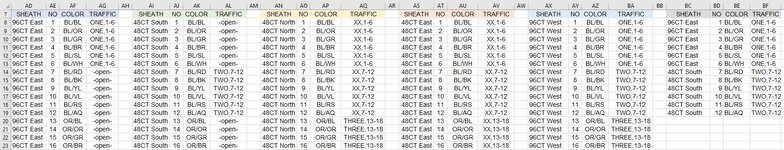
Here are the helper tables:
MrExcel_20240213b.xlsx
BNBOBPBQBRBSBTBU
1
2
3Unique Source Traffic CodesGroup 1Group 2Group 3Group 4Group 5Group 6
4ONE201000
5-open-181912121412
6TWO212112
7THREE202221
8FOUR040202
9 
10
11Cumulative Priors
12Unique STCGroup 1Group 2Group 3Group 4Group 5Group 6All Groups
13ONE0223333
14-open-0183749617587
15TWO0235679
16THREE0224689
17FOUR0044668
18
Sheet3 (2)
Cell Formulas
RangeFormula
BO4:BO8BO4=COUNTIF($U$4:$U$27,$BN4)
BP4:BP8BP4=COUNTIF($Z$4:$Z$27,$BN4)
BQ4:BQ8BQ4=COUNTIF($AG$8:$AG$24,$BN4)
BR4:BR8BR4=COUNTIF($AL$8:$AL$24,$BN4)
BS4:BS8BS4=COUNTIF($AQ$8:$AQ$24,$BN4)
BT4:BT8BT4=COUNTIF($AV$8:$AV$24,$BN4)
BN4:BN9BN4=IFERROR(INDEX($P$4:$P$34,AGGREGATE(15,6,(ROW($P$4:$P$34)-ROW($P$4)+1)/(COUNTIF($BN$3:BN3,$P$4:$P$34)=0),1)),"")
BN13:BN18BN13=BN4:BN9
BO13:BU17BO13=SUM($BN4:BN4)
Dynamic array formulas.

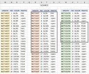
A small portion of the SourceResults table that merely copies over the original Source table:
Cell Formulas
RangeFormula
AX4:BA10AX4=INDEX($M4:$P4,1,COLUMNS($AX:AX))

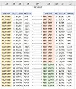
...and the corresponding small portion of the Results table that incorporates lookups in the helper table. This version would be easier to edit/maintain as each of the "group" sections of the formula are very similar.
Cell Formulas
RangeFormula
BH4:BK10BH4=IFERROR( INDEX( $R$4:$U$27, AGGREGATE(15,6, (ROW($U$4:$U$27) - ROW($U$4)+1) / ($U$4:$U$27=$BA4), COUNTIF($BA$3:$BA3,$BA4) - INDEX($BO$13:$BT$17,MATCH($BA4,$BN$13:$BN$17,0),MATCH("Group 1",$BO$12:$BT$12,0)) + 1), COLUMNS($BC:BC) ), IFERROR( INDEX( $W$4:$Z$27, AGGREGATE(15,6, (ROW($Z$4:$Z$27) - ROW($Z$4) + 1) / ($Z$4:$Z$27=$BA4), COUNTIF($BA$3:$BA3,$BA4) - INDEX($BO$13:$BT$17,MATCH($BA4,$BN$13:$BN$17,0),MATCH("Group 2",$BO$12:$BT$12,0)) + 1), COLUMNS($BC:BC) ), IFERROR( INDEX( $AD$8:$AG$24, AGGREGATE(15,6, (ROW($AG$8:$AG$24) - ROW($AG$8)+1) / ($AG$8:$AG$24=$BA4), COUNTIF($BA$3:$BA3,$BA4) - INDEX($BO$13:$BT$17,MATCH($BA4,$BN$13:$BN$17,0),MATCH("Group 3",$BO$12:$BT$12,0)) + 1), COLUMNS($BC:BC) ), IFERROR( INDEX( $AI$8:$AL$24, AGGREGATE(15,6, (ROW($AL$8:$AL$24) - ROW($AL$8)+1) / ($AL$8:$AL$24=$BA4), COUNTIF($BA$3:$BA3,$BA4) - INDEX($BO$13:$BT$17,MATCH($BA4,$BN$13:$BN$17,0),MATCH("Group 4",$BO$12:$BT$12,0)) + 1), COLUMNS($BC:BC) ), IFERROR( INDEX( $AN$8:$AQ$24, AGGREGATE(15,6, (ROW($AQ$8:$AQ$24) - ROW($AQ$8)+1) / ($AQ$8:$AQ$24=$BA4), COUNTIF($BA$3:$BA3,$BA4) - INDEX($BO$13:$BT$17,MATCH($BA4,$BN$13:$BN$17,0),MATCH("Group 5",$BO$12:$BT$12,0)) + 1), COLUMNS($BC:BC) ), IFERROR( INDEX( $AS$8:$AV$24, AGGREGATE(15,6, (ROW($AV$8:$AV$24) - ROW($AV$8)+1) / ($AV$8:$AV$24=$BA4), COUNTIF($BA$3:$BA3,$BA4) - INDEX($BO$13:$BT$17,MATCH($BA4,$BN$13:$BN$17,0),MATCH("Group 6",$BO$12:$BT$12,0)) + 1), COLUMNS($BC:BC) ), "" ))))))
 
Last edited:
Upvote 0
Okay...thanks. Give this version a try. I want to avoid the array produced by making a logical test of a range being equal to a specific value, so I've changed the SUM portion of the formula.
Cell Formulas
RangeFormula
AB4:AE11AB4=INDEX($M4:$P4,1,COLUMNS($AB:AB))
AF4:AI11AF4=IFERROR( INDEX($R$4:$U$27, AGGREGATE(15,6,(ROW($U$4:$U$27)-ROW($U$4)+1)/($U$4:$U$27=$AE4), IF(COUNTIF($AE$3:$AE3,$AE4)<(COUNTIF($U$4:$U$27,$AE4)+COUNTIF($Z$4:$Z$27,$AE4)), COUNTIF($AE$3:$AE3,$AE4)+1)),COLUMNS($AF:AF)), IFERROR( INDEX($W$4:$Z$27, AGGREGATE(15,6,(ROW($Z$4:$Z$27)-ROW($Z$4)+1)/($Z$4:$Z$27=$AE4), IF(COUNTIF($AE$3:$AE3,$AE4)<(COUNTIF($U$4:$U$27,$AE4)+COUNTIF($Z$4:$Z$27,$AE4)), COUNTIF($AE$3:$AE3,$AE4)+1)),COLUMNS($AF:AF)), ""))
Sorry I didn't get back to you sooner, its been a busy past week.
Your formula worked perfectly for what I'm trying to achieve and I can't thank you enough for all your help.
This will definitely save me a lot of time and headache so I appreciate everything you have done.

T
 
Upvote 0
You're welcome...I'm happy to help. It looks as if you might be using the version described in post #10? Do be aware of the vulnerability I mentioned in later posts. As I recall, the issue arises when the same Traffic code appears across multiple tables, and it becomes necessary to determine the cumulative count of that Traffic code across prior tables so that the correct matching Traffic codes in the current table can be delivered by the formula. This was described in greater detail in post #12, and some improvements to address the problem were shown in subsequent posts. So check carefully to confirm that the behavior is as desired.
 
Upvote 0

Forum statistics

Threads
1,215,069
Messages
6,122,954
Members
449,095
Latest member
nmaske

We've detected that you are using an adblocker.

We have a great community of people providing Excel help here, but the hosting costs are enormous. You can help keep this site running by allowing ads on MrExcel.com.
Allow Ads at MrExcel

Which adblocker are you using?

Disable AdBlock

Follow these easy steps to disable AdBlock

1)Click on the icon in the browser’s toolbar.
2)Click on the icon in the browser’s toolbar.
2)Click on the "Pause on this site" option.
Go back

Disable AdBlock Plus

Follow these easy steps to disable AdBlock Plus

1)Click on the icon in the browser’s toolbar.
2)Click on the toggle to disable it for "mrexcel.com".
Go back

Disable uBlock Origin

Follow these easy steps to disable uBlock Origin

1)Click on the icon in the browser’s toolbar.
2)Click on the "Power" button.
3)Click on the "Refresh" button.
Go back

Disable uBlock

Follow these easy steps to disable uBlock

1)Click on the icon in the browser’s toolbar.
2)Click on the "Power" button.
3)Click on the "Refresh" button.
Go back
Back
Top