Tricky counting formula

[mjones]

Hi All,

At > 6000 rows, it’s impossible to manually count so I hope a formula genius out there can help.

All cells are general format with text.

Count how many situations occur with rows with the same text in columns B, D & E that also have a row with x in column G and another row with y in column G.

The case below would count 1 for rows 1 and 2 matching the scenario, but rows 3 and 4 do not count because even though B, D & E match, there are not two rows where one has an x and one has a y in column G.

B D E G
1 AB CD EF x
2 AB CD EF y
3 GH KL TY z
4 GH KL TY y

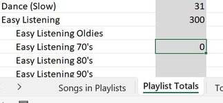
The above is in the 'Songs in Playlists'! tab, but the count/answer will be in another tab.

Thank you for considering my formula,

Michele

 

[mjones]

I'm doing this because some playlists like easy listening will have 800 songs and that's too big so I wanted to know which ones should also have separate playlists by decade.

 

[KRice]

Try the SUMPRODUCT version I posted and let me know it it’s results make sense.

 

[mjones]

Sorry for the delay, I had to go out yesterday afternoon.

I reviewed my original question and it is correct. I can't think how to explain it better.

Count how many situations occur with rows with the same text in columns B, D & E that also have a row with x in column G and another row with y in column G.

The case below would count 1 for rows 1 and 2 matching the scenario, but rows 3 and 4 do not count because even though B, D & E match, there are not two rows where one has an x and one has a y in column G.

B D E G
1 AB CD EF x
2 AB CD EF y
3 GH KL TY z
4 GH KL TY y

I know it's very tricky (thus the title of this post) and understand if it can't be done. Without the formula, it'll be very time consuming.

Thank you very much anyway,

Michele

 

[mjones]

Sorry, missed your last message.

I used =LET(src,'Songs in Playlists'!$B$2:$G$5746,s,CHOOSECOLS(src,1,3,4,6),b,CHOOSECOLS(s,1),d,CHOOSECOLS(s,2),e,CHOOSECOLS(s,3),g,CHOOSECOLS(s,6),fres,FILTER(s,(b=A3)*(d=B3)*(e=C3),EXPAND("",1,COLUMNS(s),"")),lcol,CHOOSECOLS(fres,4),xs,SUM(--(lcol="Rock")),ys,SUM(--(lcol="80's")),IF(AND(xs>0,ys>0),SUM(xs,ys),0))

which results in 0.

 

[KRice]

I'm certain this can be done, but we'll need to get the formula adjusted correctly. Let's review...you've defined the source data as "src" in 'Songs in Playlists'!$B$2:$G$5746. Confirm this worksheet name and range...in an earlier post, I understood the worksheet name has a "the" in it...'Songs in the Playlists'. The formula is taking column B there as the 1st column, C as the 2nd, and so on. So the formula takes columns 1, 3, and 4 from this src data and assigns then to variables b, d, and e, respectively. And the 6th column is assigned to "g" (where the x's and y's or Rock and 80's might be found). I don't see any issues up to this point, except possibly the worksheet name.

Then we obtain filtered results (fres) that require the b, d, and e criteria to be met. And if nothing is found, a four-column empty array (blanks) is returned (that's what the EXPAND function does). Then we take the last column of fres (where the x's and y's are found)...and we call this last column "lcol" for convenience. We then sum the number of matches in lcol to determine how many ="Rock" (that's xs), and how many ="80's" (that's ys). We want to confirm that at least one of each is found, which would mean that at least a matching pair was found (where b, d, e are the same AND one of column g is an "x" AND one of column of g is a "y"). The minimum of the sums found represents the number of matching pairs....so change the last "SUM" in the formula to "MIN" (I think I suggested that in an earlier post).

But if you're showing 0 right now, the SUM/MIN isn't the issue...it's something else, so let me know about the worksheet name question.

 

[mjones]

Hi KRice,

'Songs in Playlists'!$B$2:$G$5746 is correct. My first post didn’t have ‘the’ and I’ve done it correctly in all tests.

From the source data (B to G, now src 1, 3, 4, 6 which ignores columns C and F),
- B is the 1st column (song name),
- D is the 2nd column (artist),
- E is the 3rd column (album), and
- G is the 4th column (playlist, e.g. Rock or 80’s).

So yes, columns 1, 3, and 4 from this src data could reasonably be assigned as you say.

Yes, we want to confirm that at least one of each in column G (4) is found, which would mean that at least a matching pair was found where b, d, e are the same.

I changed the last SUM to MIN like this:

=LET(src,'Songs in Playlists'!$B$2:$G$5746,s,CHOOSECOLS(src,1,3,4,6),b,CHOOSECOLS(s,1),d,CHOOSECOLS(s,2),e,CHOOSECOLS(s,3),g,CHOOSECOLS(s,6),fres,FILTER(s,(b=A3)*(d=B3)*(e=C3),EXPAND("",1,COLUMNS(s),"")),lcol,CHOOSECOLS(fres,4),xs,SUM(--(lcol="Rock")),ys,SUM(--(lcol="80's")),IF(AND(xs>0,ys>0),MIN(xs,ys),0))

And still get zero. The result cell is general format. Changing it to number results in 0.00.

You seem to have a good understanding so I’m stumped.

Michele

 

[KRice]

Does column G in the 'Songs in Playlists' worksheet contain only "Rock" for those rows that should be considered? For example, it doesn't say "Soft Rock" or "Hard Rock". An exact match is expected. Same with "80's"...an exact match?

 

[mjones]

I apologize, I have a commitment and have to go out so if I don't reply right away, that's the reason. Thanks again!

 

[KRice]

No problem. Here is what I would do if I had access to your workbook...
Drag the formula that is supposed to perform the pair counting to the right where you have an empty column and several more empty columns to its right. And then modify the formula (or pasted this one directly in that cell). The one shown here uses terms in F3 and G3 for matching...Rock and 80's in your example. You can either use this idea, or hardwire those terms inside quotation marks into the formula:

=LET(src,'Songs in Playlists'!$B$1:$G$12,
s,CHOOSECOLS(src,1,3,4,6), b,CHOOSECOLS(s,1), d,CHOOSECOLS(s,2), e,CHOOSECOLS(s,3), g,CHOOSECOLS(s,6),
fres,FILTER(s,(b=A3)*(d=B3)*(e=C3),EXPAND("",1,COLUMNS(s),"")), lcol,CHOOSECOLS(fres,4), xs,SUM(--(lcol=F3)), ys,SUM(--(lcol=G3)), res, IF(AND(xs>0,ys>0),MIN(xs,ys),0), lcol)

I've modified the last part of the formula by assigning the current end result to a variable called "res". Then at the very end of the formula, you can type any of the prior variable names to see what they look like...if they are arrays, they will spill down and to the right, depending on whether they are one or two-dimensional arrays, horizontal and vertical. If you want to see the final count, enter "res"...to check what the vertical matching array looks like for the part of the formula inside the FILTER function where we want to match (b=A3), just enter that (b=A3) at the end of the formula, etc. In the latter case, you'll see a very long vertical array of TRUEs and FALSEs indicating row-by-row whether the items in the b array match the value in A3. For debugging purposes, I would recommend setting your "src" to maybe 20-30 rows and confirm by inspection that you have at least a matching pair. Then set the match terms in your results sheet so that you should find that particular result. Then interrogate the formula terms by term to determine where it is failing. I suspect there may be some extra spaces or hidden characters in the text that are preventing matches, but I'm only guessing.

To illustrate, using the same sample date shown in my post #6, except I've changed the worksheet name now to 'Songs in Playlists', here is what I get when I drag the formula in D3 over to cell I3 and instruct the formula to show the intermediate filtered results (fres). I can see that all of the b, d, and e matches were found, spilled down and to the right from cell I3 (that is AB was found in array b, CD was found in array d, and ER was found in array e). Looking at the 4th column in fres, one result matches one of the final search terms, and two results match the other final search term...so the final result will be 1...one pair.

MrExcel_20240301.xlsx
	A	B	C	D	E	F	G	H	I	J	K	L
1
2	CatB	CatD	CatE	Pair Count
3	AB	CD	EF			Oldies (Pre 1970)	Easy Listening/'Smooth' Jazz		AB	CD	EF	Oldies (Pre 1970)
4	GH	KL	TY	2		Oldies (Pre 1970)	Easy Listening/'Smooth' Jazz		AB	CD	EF	Easy Listening/'Smooth' Jazz
5	GH	KL	AB	0		Oldies (Pre 1970)	Easy Listening/'Smooth' Jazz		AB	CD	EF	Easy Listening/'Smooth' Jazz
6									AB	CD	EF	q
mjones_tab

Cell Formulas
Range	Formula
I3:L6	I3	=LET(src,'Songs in Playlists'!$B$1:$G$12, s,CHOOSECOLS(src,1,3,4,6), b,CHOOSECOLS(s,1), d,CHOOSECOLS(s,2), e,CHOOSECOLS(s,3), g,CHOOSECOLS(s,6), fres,FILTER(s,(b=A3)*(d=B3)*(e=C3),EXPAND("",1,COLUMNS(s),"")), lcol,CHOOSECOLS(fres,4), xs,SUM(--(lcol=F3)), ys,SUM(--(lcol=G3)), res, IF(AND(xs>0,ys>0),MIN(xs,ys),0), fres)
D4:D5	D4	=LET(src,'Songs in Playlists'!$B$1:$G$12, s,CHOOSECOLS(src,1,3,4,6), b,CHOOSECOLS(s,1), d,CHOOSECOLS(s,2), e,CHOOSECOLS(s,3), g,CHOOSECOLS(s,6), fres,FILTER(s,(b=A4)*(d=B4)*(e=C4),EXPAND("",1,COLUMNS(s),"")), lcol,CHOOSECOLS(fres,4), xs,SUM(--(lcol=F4)), ys,SUM(--(lcol=G4)), IF(AND(xs>0,ys>0),MIN(xs,ys),0))
Dynamic array formulas.

If your file doesn't have anything sensitive in it, and you are willing to share it, you could upload it to a common file sharing site (Dropbox, Box, etc.) and share the link...and I could have a look to determine what is causing the problem.

 

[mjones]

I just wanted to let you to know I got your message above. It's past 7 here and dinner time so when my brain is rested tomorrow, I'll dive into it. I have a website and can probably put the file up there for you to get but because I'm just retired and about to get rid of the website, I have to find the application to upload it but I'll try.