Multiple Conditions - Conditional Format

[TAPS_MikeDion]

Hi everyone,
I know how to do most conditional formatting, but this one I'm not sure of. Hopefully I can explain it well enough so you understand what I'm looking for.

Could someone please figure out a formula that checks for the following?

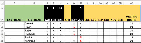
• With cells S3 - AD100, if there is no "x" in the cell, but there is a value>0 in the cell S1 - AD1, then I need to highlight the fill of the cell

By looking at the attached image you'll see that cell U7 has no x, but there is a value greater than 0 in cell U1. The formatting would then highlight the fill color of that cell.

Thank you for any help offered!

 

[Joe4]

Select cells S1:AD1 and enter this Conditional Formatting formula:

=and(countif(S3:S100,"x")=0,S1>0)

and choose your desired formatting color.

 

[JamesCanale]

MrExcelPlayground18.xlsx
	S	T	U	V	W
1	5	12		7	4
2	Feb	Mar	Apr	May	June
3	x	x		x	x
4	x	x		5	x
5	x			x	x
6	x	x		5	x
Sheet2

Cells with Conditional Formatting
Cell	Condition		Cell Format	Stop If True
S3:W6	Expression	=AND(S3<>"x",S$1>0)	text	NO

 

[Joe4]

MrExcelPlayground18.xlsx
	S	T	U	V	W
1	5	12		7	4
2	Feb	Mar	Apr	May	June
3	x	x		x	x
4	x	x		5	x
5	x			x	x
6	x	x		5	x
Sheet2

Cells with Conditional Formatting
Cell	Condition		Cell Format	Stop If True
S3:W6	Expression	=AND(S3<>"x",S$1>0)	text	NO

James, I had to re-read that a few times to fully grasp it myself, but I am pretty sure that they only want to apply the Conditional Formatting to row 1, not each data row, based on the condition that no "x"s appear in rows 3-100 for that particular column, and there is a number > 0 in row 1 of that column.

 

[JamesCanale]

Ambiguous antecedents for "the cell"

I expect he will have what he needs one way or the other.

 

[TAPS_MikeDion]

Hi James & Joe,
I haven't tried either of your suggestions yet, but the cells that I need to have the conditional formatting highlight are from S3 to AD100, but only if the cell(s) S3 to AD100 do not contain an "x" and the cell above it (S1 to AD1) has a value greater than 0.

I hope that helps a little more.

 

[TAPS_MikeDion]

James, I tried your formula and it is doing what I need, except that it is also highlighting cells from S3 to AD100 which contain a number. It must only apply if the cell is blank.

Thank you!

 

[TAPS_MikeDion]

Got it, James. I just changed your formula to S3="" and it works perfectly! Thank you!