Need formula range to automatically expand when a new row is added to table

[Mike423]

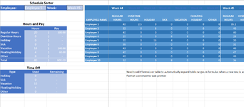
I'm currently using the below formula to sum individual payroll values from a large table into a smaller, summary table.

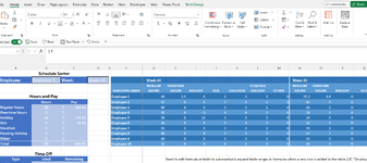
=IF(D2="YTD",SUMPRODUCT((G4:BQ13)*(G3:BQ3=A6)*(F4:F13=B2)),SUMPRODUCT((G4:BQ13)*(F4:F13=B2)*(G2:BQ2=D2)*(G3:BQ3=A6)))

My question is, how can I modify this formula, so that when I drag the bottom row of the table down (it is actually a table, not just a range) to add a new row, the ranges in the formula adjust along with it to include any data entered into the new row? Picture is attached.

Thank you.

 

[KRice]

Since you have an official table already, I recommend using structured references in the formula. The formula would then use the column names, and a formula entered in the top cell of the column will apply down...even as new rows are added.

Book1
	A	B	C	D
1	Employee Name	Regular Hours	Overtime Hours	Total Hours
2	Emp 1	40	2	42
3	Emp 2	32	1	33
4				0
5				0
Sheet1

Cell Formulas
Range	Formula
D2:D5	D2	=SUM(Table1[@[Regular Hours]:[Overtime Hours]])

Using structured references with Excel tables - Microsoft Support

Structured references make it easier to use formulas with Excel tables by replacing cell references, such as C2:C7, with predefined names for the items in a table.

support.microsoft.com

 

[KRice]

Here is a small working example based on the screenshot you posted that illustrates how the structured reference approach could be used. Note that Excel will not allow multiple columns to have the same name in an actual table, so the default behavior has Excel appending a number to the end of the heading. That creates a problem in this case because you want to match column headings to "Regular Hours". I opted to create this match by using the leftmost 7 characters. Speaking of problems, the (G2:BQ2=D2)*(G3:BQ3=A6) in your original formula is likely to cause a problem because you appear to want to match both the week number and the column "Regular Hours", but if those two labels are not in the same column, this construction will not permit either column to be considered. So I've assumed that the week number and "Regular Hours" will always be in the same column, therefore, the formula needs to consider only one of them. If you want to extract other types of hours from the data table, a somewhat modified approach would be necessary to account for how far those columns are from the week number label.

Book1
	A	B	C	D	E	F	G	H	I	J	K	L	M	N	O	P	Q	R	S	T
1						79
2	Employee:	Emp 1	Week:	YTD			Week 44							Week 45
3						Employee Name	Regular Hours	Overtime Hours	Holiday	Sick	Vacation	Floating Holiday	Other	Regular Hours2	Overtime Hours2	Holiday2	Sick2	Vacation2	Floating Holiday2	Other2
4						Emp 1	40	2						39	2
5		Hours	Pay			Emp 2	32	1						33	1
6	Regular Hours	20	300			Emp 3	41	4						22	4
7	Overtime Hours
8	Holiday
9	Sick
10	Vacation	16	240
11	Floating Holiday
12	Other
Sheet1

Cell Formulas
Range	Formula
F1	F1	=IF($D$2="YTD", SUM(FILTER(FILTER(Table1[#Data],LEFT(Table1[#Headers],7)=LEFT($A$6,7)),Table1[Employee Name]=$B$2)), FILTER(FILTER(Table1[#Data],OFFSET(Table1[#Headers],-1,)=$D$2),Table1[Employee Name]=$B$2))

 

[Mike423]

Thanks for the response! I should have mentioned that each week section has the week name in every cell above the section, so week 44 has week 44 above regular hours, overtime hours, etc, its just hidden in all but the first column. Do the weeks pay type column headers absolutely have to be appended with their own specific number? Seems most of the problems stem from the fact that I've made this a table already. I've tried a series of different formulas like the one you provided but have not yet been able to make it work. Any additional advice would be very much appreciated!

 

[KRice]

Thanks for the clarification about the week number labels...in that case, your original formula does handle those two conditions correctly (matching "Regular Hours" and the appropriate week number). I don't understand how you can have an official "table" if you have duplicate column headings. If you click anywhere in the "table", does "Table Design" appear in the upper menu (where you'll find File, Home, Insert, Draw, etc. typically)? For now, I've converted the table range back to a normal range, so duplicate column headers are permitted. Then, because you do not have the benefit of the formula adapting to a changing table size, you can dynamically determine the size of the data array with formulas. That's somewhat more complicated, but it should offer the same flexibility in that the formula does not require further editing if the table expands to the right or down, or both. Give it a try to see if it suits your needs better.

I've left some formulas in X5:X6 so that you can see what they do (determine the row and column numbers of the last non-empty cell in column F and row 3). That approach is used to determine where the lower right corner of your data table is. So the formula requires you to specify the upper left corner of the data table (F4 where Employee 1 is named), and then confirm that your header 1 (on row 2) and header 2 (on row 3) have the correct starting cell (F2 and F3 in this example). The formulas should then create arrays of each of the two header rows and a two-dimensional array of your data table, all of which are used by the earlier formula to perform the data filtering and final sum.

Regarding your question about column names in a table...each column heading must be unique, so it is not necessary to append a number to similar headings. But they need to be different in some way. Since this approach uses a range rather than a table, duplicate headings are permitted.

MrExcel_20231030_B.xlsx
	A	B	C	D	E	F	G	H	I	J	K	L	M	N	O	P	Q	R	S	T	U	V	W	X
1			Reg Hrs	40
2	Employee:	Emp 1	Week:	Week 45			Week 44	Week 44	Week 44	Week 44	Week 44	Week 44	Week 44	Week 45	Week 45	Week 45	Week 45	Week 45	Week 45	Week 45
3						Employee Name	Regular Hours	Overtime Hours	Holiday	Sick	Vacation	Floating Holiday	Other	Regular Hours	Overtime Hours	Holiday	Sick	Vacation	Floating Holiday	Other
4						Emp 1	40	2						39	2							Helper Lists
5		Hours	Pay			Emp 2	32	1						33	1							YTD	Emp 0	9
6	Regular Hours	20	300			Emp 3	41	4						22	4							Week 44	Emp 1	20
7	Overtime Hours					Emp 1	3	2						1	2							Week 45	Emp 2
8	Holiday																						Emp 3
9	Sick					Emp 0	11	4						17	4
10	Vacation	16	240
11	Floating Holiday
12	Other
Sheet3

Cell Formulas
Range	Formula
D1	D1	=LET( maxrow,LOOKUP(2,1/--(F:F<>""),ROW(F:F)), maxcol,LOOKUP(2,1/--(3:3<>""),COLUMN(3:3)), datarng,$F$4:INDEX($1:$1048576,maxrow,maxcol), header1,$F$2:INDEX($1:$1048576,2,maxcol), header2,$F$3:INDEX($1:$1048576,3,maxcol), IF($D$2="YTD", SUM(FILTER(FILTER(datarng,header2=$A$6),INDEX(datarng,,1)=$B$2)), SUM(FILTER(FILTER(datarng,(header2=$A$6)*(header1=$D$2)),INDEX(datarng,,1)=$B$2))))
V5:V7	V5	=LET(lst,TRANSPOSE(SORT(UNIQUE(OFFSET(Sheet3!$F$3:$T$3,-1,),TRUE))),wks,FILTER(lst,lst<>""),VSTACK("YTD",wks))
W5:W8	W5	=LET(elst,SORT(UNIQUE(Sheet3!$F$4:$F$12)),FILTER(elst,elst<>""))
X5	X5	=LOOKUP(2,1/--(F:F<>""),ROW(F:F))
X6	X6	=LOOKUP(2,1/--(3:3<>""),COLUMN(3:3))
Dynamic array formulas.

Cells with Data Validation
Cell	Allow	Criteria
B2	List	=$W$5#
D2	List	=$V$5#

 

[Mike423]

Yes, "Table Design" does show up when I click on any cell within the large table area. I've attached a screenshot, which of course doesn't show a cell highlighted since I used the snipping tool to take the picture, buy you can see the table design option at the top of the screen. Is there a formula that would work with this table, that has duplicated column headers?
Thanks again.

 

[KRice]

Interesting. Click on the name "Employee 1" name in the table and then go to Table Design, and look in the Properties sub-menu where you have the option to "Resize Table". When you click on Resize Table, you'll see a new popup box with the current table range shown. What is that range reference? I'm curious about whether you might have a table without headers, in which case Excel will by default assign names of Column1, Column2, etc. And if you hide that row and then type your own column headings (that are not actually part of the official table), you could still produce a table that looks like what you've posted, including apparent duplicate column names. Could you tell me the row numbers appearing on the left side of the screen that correspond to the cells where "Week 44", "Employee Name", and "Employee 1" appear?

As for a potential solution, have you tried out my last post? I think that should work. Alternatively, depending on your answer to my table range reference questions, there may be another way forward.

 

[Mike423]

Here are the table dimensions: $F$2:$BQ$13
Week 44: Row 2
Employee Name: Row 3
Employee 1: Row 4

 

[KRice]

Oh…so the table begins on row 2? What text appears in the column headings moving across row 2?

 

[Mike423]

"Week 44" G2 through M2, then "Week 45" N2 through T2 and so on. So the week number in each cell on row 2 above the week's section.