Not sure what formula to use.... Index match, Vlookup or ?

[SelinaR]

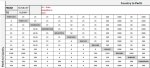
I have a mileage chart that runs on an x and a y-axis and need to have a drop-down that picks up a TO and FROM but in the correct axis.

I have tried multiple options but because the data has two prices (city to country and country to the city) I can't find a solution.

I have made a drop-down box for from and to but as there are two sets of data, how can I build a formula to pick up the correct axis.?

Thanks so much in advance for your help

 

[lrobbo314]

what would the correct value for the example in the picture, Albany to Bunbury? 300, 350, 650?

 

[SelinaR]

what would the correct value for the example in the picture, Albany to Bunbury? 300, 350, 650?

Albany to Bunbury = 350 (down and across to the right)
AND
Bunbury to Albany = 300 (up and across (to the left)

 

[lrobbo314]

Here are a couple of options.

VBA

20200910 MXL Intersect.xlsm
	B	C	D	E	F	G	H	I	J	K	L	M
2	From	ALBANY	300
3	To	BUNBURY	350
4	PERTH APO	85	560	580	199	170	59	611	550	393	68	245
5	0	PERTH CITY	254	95	249	111	665	150	714	794	583	763
6	25	943	FREEMANTLE	580	679	899	636	936	369	587	286	24
7	25	153	677	OSBORNE PARK	151	461	978	404	749	503	32	297
8	25	302	966	814	WELSHPOOL	717	339	633	530	346	575	360
9	25	981	20	596	45	WANGARA	636	670	707	194	472	333
10	25	367	701	422	944	118	REDCLIFF	892	1	734	108	340
11	300	398	974	491	914	970	292	MIDLAND	124	834	438	399
12	1000	152	357	395	608	825	285	217	ALBANY	119	300	839
13	90	367	812	951	313	376	177	851	601	BROOME	358	110
14	750	996	79	588	814	579	672	344	350	307	BUNBURY	804
15	450	783	338	355	444	42	88	10	557	380	560	CARNARVON
Sheet1

'Worksheet Code
Private Sub Worksheet_Change(ByVal Target As Range)
If Not Intersect(Range("C2:C3"), Target) Is Nothing Then Dist
End Sub

'Standard Module
Sub Dist()
Dim r As Range:         Set r = Range("B4:M" & Range("B" & Rows.Count).End(xlUp).Row)
Dim iFrom As String:    iFrom = Range("C2").Value
Dim iTo As String:      iTo = Range("C3").Value
Dim fCel As Range:      Set fCel = r.Find(iFrom, r.Cells(1), xlValues, xlWhole)
Dim sCel As Range:      Set sCel = r.Find(iTo, r.Cells(1), xlValues, xlWhole)

Range("D2").Value = Application.Intersect(Range(Rows(fCel.Row).Address), Range(Columns(sCel.Column).Address))
Range("D3").Value = Application.Intersect(Range(Rows(sCel.Row).Address), Range(Columns(fCel.Column).Address))
End Sub

Power Query

20200910 MXL Intersect.xlsm
	O	P
2	City	Dist
3	REDCLIFF	340
4	CARNARVON	88
Sheet1

(city1 as text, city2 as text) as table =>

let
    Source = Excel.CurrentWorkbook(){[Name="Table2"]}[Content],
    Unpivot = Table.UnpivotOtherColumns(Source, {}, "Attribute", "Value"),
    GroupCol = Table.AddColumn(Unpivot, "Custom", each if Value.Is([Value], type text) then [Value] else null),
    FilledDown = Table.FillDown(GroupCol,{"Custom"}),
    ColumnCol = Table.AddColumn(FilledDown, "Column", each if [Value]=[Custom] then [Attribute] else null),
    Group = Table.Group(ColumnCol, {"Custom"}, {{"Count", each _, type table}}),
    cID = Table.AddIndexColumn(Group, "cID", 0, 1),
    RC = Table.RemoveColumns(cID,{"cID"}),
    iFrom = RC{cID{[Custom=city1]}[cID]}[Count][Column]{0},
    iTo = RC{cID{[Custom=city2]}[cID]}[Count][Column]{0},
    c1 = cID{[Custom=city1]}[cID],
    c2 = cID{[Custom=city2]}[cID]-1,
    Result = Table.FromRecords({[City=RC{c1}[Count]{[Attribute=iTo]}[Custom], Dist=RC{c1}[Count]{[Attribute=iTo]}[Value]],[City=RC{c2+1}[Count]{0}[Value],Dist=RC{c2}[Count]{[Attribute=iFrom]}[Value]]})
in
    Result

The Power query code is a custom function that you invoke by entering in the 2 city names that you want to look up.

 

[lrobbo314]

Here's a formula solution as well.

20200910 MXL Intersect.xlsm
	B	C	D	E	F	G	H	I	J	K	L	M
2	From	WELSHPOOL	346	346
3	To	BROOME	313	313
4	PERTH APO	85	560	580	199	170	59	611	550	393	68	245
5	0	PERTH CITY	254	95	249	111	665	150	714	794	583	763
6	25	943	FREEMANTLE	580	679	899	636	936	369	587	286	24
7	25	153	677	OSBORNE PARK	151	461	978	404	749	503	32	297
8	25	302	966	814	WELSHPOOL	717	339	633	530	346	575	360
9	25	981	20	596	45	WANGARA	636	670	707	194	472	333
10	25	367	701	422	944	118	REDCLIFF	892	1	734	108	340
11	300	398	974	491	914	970	292	MIDLAND	124	834	438	399
12	1000	152	357	395	608	825	285	217	ALBANY	119	300	839
13	90	367	812	951	313	376	177	851	601	BROOME	358	110
14	750	996	79	588	814	579	672	344	350	307	BUNBURY	804
15	450	783	338	355	444	42	88	10	557	380	560	CARNARVON
Sheet1

Cell Formulas
Range	Formula
E2	E2	=INDEX(City,SUMPRODUCT(($B$4:$M$15=C2)*ROW($B$4:$M$15))-3,SUMPRODUCT(($B$4:$M$15=C3)*ROW($B$4:$M$15))-3)
E3	E3	=INDEX(City,SUMPRODUCT(($B$4:$M$15=C3)*ROW($B$4:$M$15))-3,SUMPRODUCT(($B$4:$M$15=C2)*ROW($B$4:$M$15))-3)

 

[Fluff]

If you are happy to change the data slightly, you could use this simpler formula

+Fluff New.xlsm
	A	B	C	D	E	F	G	H	I	J	K	L	M	N
1
2		From	Albany	350
3		To	Bunbury
4			PERTH APO	PERTH CITY	FREEMANTLE	OSBORNE PARK	WELSHPOOL	WANGARA	REDCLIFF	MIDLAND	ALBANY	BROOME	BUNBURY	CARNARVON
5		PERTH APO		85	560	580	199	170	59	611	550	393	68	245
6		PERTH CITY	0		254	95	249	111	665	150	714	794	583	763
7		FREEMANTLE	25	943		580	679	899	636	936	369	587	286	24
8		OSBORNE PARK	25	153	677		151	461	978	404	749	503	32	297
9		WELSHPOOL	25	302	966	814		717	339	633	530	346	575	360
10		WANGARA	25	981	20	596	45		636	670	707	194	472	333
11		REDCLIFF	25	367	701	422	944	118		892	1	734	108	340
12		MIDLAND	300	398	974	491	914	970	292		124	834	438	399
13		ALBANY	1000	152	357	395	608	825	285	217		119	300	839
14		BROOME	90	367	812	951	313	376	177	851	601		358	110
15		BUNBURY	750	996	79	588	814	579	672	344	350	307		804
16		CARNARVON	450	783	338	355	444	42	88	10	557	380	560
Master

Cell Formulas
Range	Formula
D2	D2	=INDEX(C5:N16,MATCH(C3,B5:B16,0),MATCH(C2,C4:N4,0))

 

[lrobbo314]

In my previous solution I failed to mention that I used a named range for B4:M15. I also didn't replace all the range references.

20200910 MXL Intersect.xlsm
	B	C	D	E	F	G	H	I	J	K	L	M
2	From	WELSHPOOL	339	339
3	To	REDCLIFF	944	944
4	PERTH APO	85	560	580	199	170	59	611	550	393	68	245
5	0	PERTH CITY	254	95	249	111	665	150	714	794	583	763
6	25	943	FREEMANTLE	580	679	899	636	936	369	587	286	24
7	25	153	677	OSBORNE PARK	151	461	978	404	749	503	32	297
8	25	302	966	814	WELSHPOOL	717	339	633	530	346	575	360
9	25	981	20	596	45	WANGARA	636	670	707	194	472	333
10	25	367	701	422	944	118	REDCLIFF	892	1	734	108	340
11	300	398	974	491	914	970	292	MIDLAND	124	834	438	399
12	1000	152	357	395	608	825	285	217	ALBANY	119	300	839
13	90	367	812	951	313	376	177	851	601	BROOME	358	110
14	750	996	79	588	814	579	672	344	350	307	BUNBURY	804
15	450	783	338	355	444	42	88	10	557	380	560	CARNARVON
Sheet1

Cell Formulas
Range	Formula
E2	E2	=INDEX(City,SUMPRODUCT((City=C2)*ROW(City))-3,SUMPRODUCT((City=C3)*ROW(City))-3)
E3	E3	=INDEX(City,SUMPRODUCT((City=C3)*ROW(City))-3,SUMPRODUCT((City=C2)*ROW(City))-3)

 

[SelinaR]

Hiya - thanks for this I will try the various option provided

 

[SelinaR]

If you are happy to change the data slightly, you could use this simpler formula

+Fluff New.xlsm
	A	B	C	D	E	F	G	H	I	J	K	L	M	N
1
2		From	Albany	350
3		To	Bunbury
4			PERTH APO	PERTH CITY	FREEMANTLE	OSBORNE PARK	WELSHPOOL	WANGARA	REDCLIFF	MIDLAND	ALBANY	BROOME	BUNBURY	CARNARVON
5		PERTH APO		85	560	580	199	170	59	611	550	393	68	245
6		PERTH CITY	0		254	95	249	111	665	150	714	794	583	763
7		FREEMANTLE	25	943		580	679	899	636	936	369	587	286	24
8		OSBORNE PARK	25	153	677		151	461	978	404	749	503	32	297
9		WELSHPOOL	25	302	966	814		717	339	633	530	346	575	360
10		WANGARA	25	981	20	596	45		636	670	707	194	472	333
11		REDCLIFF	25	367	701	422	944	118		892	1	734	108	340
12		MIDLAND	300	398	974	491	914	970	292		124	834	438	399
13		ALBANY	1000	152	357	395	608	825	285	217		119	300	839
14		BROOME	90	367	812	951	313	376	177	851	601		358	110
15		BUNBURY	750	996	79	588	814	579	672	344	350	307		804
16		CARNARVON	450	783	338	355	444	42	88	10	557	380	560
Master

Cell Formulas
Range	Formula
D2	D2	=INDEX(C5:N16,MATCH(C3,B5:B16,0),MATCH(C2,C4:N4,0))

Hiya - thanks for this one... I previously tried to use this option, but as the $ are different from and to and then to and from it wasn't accurate

 

[SelinaR]

In my previous solution I failed to mention that I used a named range for B4:M15. I also didn't replace all the range references.

20200910 MXL Intersect.xlsm
	B	C	D	E	F	G	H	I	J	K	L	M
2	From	WELSHPOOL	339	339
3	To	REDCLIFF	944	944
4	PERTH APO	85	560	580	199	170	59	611	550	393	68	245
5	0	PERTH CITY	254	95	249	111	665	150	714	794	583	763
6	25	943	FREEMANTLE	580	679	899	636	936	369	587	286	24
7	25	153	677	OSBORNE PARK	151	461	978	404	749	503	32	297
8	25	302	966	814	WELSHPOOL	717	339	633	530	346	575	360
9	25	981	20	596	45	WANGARA	636	670	707	194	472	333
10	25	367	701	422	944	118	REDCLIFF	892	1	734	108	340
11	300	398	974	491	914	970	292	MIDLAND	124	834	438	399
12	1000	152	357	395	608	825	285	217	ALBANY	119	300	839
13	90	367	812	951	313	376	177	851	601	BROOME	358	110
14	750	996	79	588	814	579	672	344	350	307	BUNBURY	804
15	450	783	338	355	444	42	88	10	557	380	560	CARNARVON
Sheet1

Cell Formulas
Range	Formula
E2	E2	=INDEX(City,SUMPRODUCT((City=C2)*ROW(City))-3,SUMPRODUCT((City=C3)*ROW(City))-3)
E3	E3	=INDEX(City,SUMPRODUCT((City=C3)*ROW(City))-3,SUMPRODUCT((City=C2)*ROW(City))-3)

did you name the C2 and C3 cells as "city" ???