Not sure where to start...

[Hartley16]

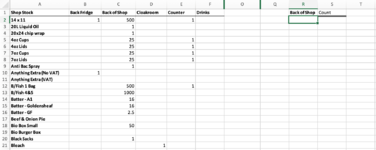
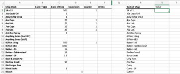
Hi, I'm hoping someone here can help me. I am trying to return the cells that have a value in column A if R1 matches with the corresponding table header. I think an array index match formula is the way to go but I can't seem to get my head around it.

 

[Fluff]

Hi & welcome to MrExcel.
Do you mean te values from col A where col C has a value?

 

[Eric W]

Welcome to MrExcel!

Your question is not entirely clear, but maybe something like this?

Book4
	A	B	C	D	E	F									O		Q	R	S
1	Shop Stock	Back Fridge	Back of Shop	Cloakroom	Counter	Drinks												Back of Shop	Count
2	A		500		1													A	15
3	B		1															B
4	C		1															C
5	D		25		1													D
6	E		25		1													E
7	F		25		1													F
8	G		25		1													G
9	H		1															H
10	I	1																K
11	J																	L
12	K		500		1													M
13	L		1000															N
14	M		16															O
15	N		16															Q
16	O		2.5															S
17	P
18	Q		50
19	R
20	S		1
21	T			1
Sheet3

Cell Formulas
Range	Formula
R2:R16	R2	=FILTER(A2:A21,INDEX(B2:F21,0,MATCH(R1,B1:F1,0))<>"")
S2	S2	=ROWS(R2#)
Dynamic array formulas.

 

[Hartley16]

Welcome to MrExcel!

Your question is not entirely clear, but maybe something like this?

Book4
	A	B	C	D	E	F									O		Q	R	S
1	Shop Stock	Back Fridge	Back of Shop	Cloakroom	Counter	Drinks												Back of Shop	Count
2	A		500		1													A	15
3	B		1															B
4	C		1															C
5	D		25		1													D
6	E		25		1													E
7	F		25		1													F
8	G		25		1													G
9	H		1															H
10	I	1																K
11	J																	L
12	K		500		1													M
13	L		1000															N
14	M		16															O
15	N		16															Q
16	O		2.5															S
17	P
18	Q		50
19	R
20	S		1
21	T			1
Sheet3

Cell Formulas
Range	Formula
R2:R16	R2	=FILTER(A2:A21,INDEX(B2:F21,0,MATCH(R1,B1:F1,0))<>"")
S2	S2	=ROWS(R2#)
Dynamic array formulas.

Thanks Eric, that's exactly what I was looking for!

 

[Eric W]

Glad we could help! Thanks for the update.

 

[Hartley16]

Glad we could help! Thanks for the update.

I now need to return the appropriate value for each item into column S so S2 should be 500, S3 should be 1 etc. What formula could I use for this?

Thanks for your help, I'm new to this

 

[Eric W]

This should work:

Book4
	A	B	C	D	E	F									O		Q	R	S	T
1	Shop Stock	Back Fridge	Back of Shop	Cloakroom	Counter	Drinks												Back of Shop		Count
2	A		500		1													A	500	15
3	B		1															B	1
4	C		1															C	1
5	D		25		1													D	25
6	E		25		1													E	25
7	F		25		1													F	25
8	G		25		1													G	25
9	H		1															H	1
10	I	1																K	500
11	J																	L	1000
12	K		500		1													M	16
13	L		1000															N	16
14	M		16															O	2.5
15	N		16															Q	50
16	O		2.5															S	1
17	P
18	Q		50
19	R
20	S		1
21	T			1
Sheet3

Cell Formulas
Range	Formula
R2:S16	R2	=FILTER(CHOOSE({1,2},A2:A21,INDEX(B2:F21,0,MATCH(R1,B1:F1,0))),INDEX(B2:F21,0,MATCH(R1,B1:F1,0))<>"")
T2	T2	=ROWS(R2#)
Dynamic array formulas.

This can be shortened a bit with LET, but Fluff will have to help you with that if you're interested, since my version of Excel doesn't have LET yet.

 

[Hartley16]

Wow, you know your stuff!

 

[lrobbo314]

Using 'Let'.

ExpandIP.xlsm
	A	B	C	D	E	F	G							N	O	P	Q	R	S	T
1	Shop Stock	Back Fridge	Back of Shop	Cloakroom	Counter	Drinks												Back of Shop	#	Count
2	14 x 11	1	500		1													14 x 11	500	15
3	20L Liquid Oil		1															20L Liquid Oil	1
4	20x24 chip wrap		1															20x24 chip wrap	1
5	4 oz cups		25		1													4 oz cups	25
6	4 oz lids		25		1													4 oz lids	25
7	7 oz cups		25		1													7 oz cups	25
8	7 oz lids		25		1													7 oz lids	25
9	Antu Bac Spray		1															Antu Bac Spray	1
10	Anything Extra (No VAT)	1																B/Fish 1 Bag	500
11	Anything Extra (VAT)																	B/Fish 4&5	1000
12	B/Fish 1 Bag		500		1													Batter - A1	16
13	B/Fish 4&5		1000															Batter - Goldensheaf	16
14	Batter - A1		16															Batter -GF	2.5
15	Batter - Goldensheaf		16															Bio Box Small	50
16	Batter -GF		2.5															Black Sacks	1
17	Beef & Onion Pue																	Total:	2188.5
18	Bio Box Small		50
19	Bio Burger Box
20	Black Sacks		1	1
21	Bleach
Sheet11

Cell Formulas
Range	Formula
R2:S17	R2	=LET(a,A2:A21,c,INDEX(B2:F21,,MATCH(R1,B1:F1)),tbl,FILTER(CHOOSE({1,2},a,c),c>0),IFERROR(INDEX(tbl,SEQUENCE(ROWS(tbl)+1),{1,2}),CHOOSE({1,2},"Total:",SUM(c))))
T2	T2	=COUNT(R2#)-1
Dynamic array formulas.

 

[Fluff]

Another option

+Fluff 1.xlsm
	A	B	C	D	E	F	G										Q	R	S
1	Shop Stock	Back Fridge	Back of Shop	Cloakroom	Counter	Drinks												Back of Shop
2	A		500		1													A	500
3	B		1															B	1
4	C		1															C	1
5	D		25		1													D	25
6	E		25		1													E	25
7	F		25		1													F	25
8	G		25		1													G	25
9	H		1															H	1
10	I	1																K	500
11	J																	L	1000
12	K		500		1													M	16
13	L		1000															N	16
14	M		16															O	2.5
15	N		16															Q	50
16	O		2.5															S	1
17	P
18	Q		50
19	R
20	S		1
21	T			1
22
23
Data

Cell Formulas
Range	Formula
R2:S16	R2	=LET(Fltr,FILTER(A2:F21,(COLUMN(A1:F1)=1)+(COLUMN(A1:F1)=MATCH(R1,A1:F1,0))),FILTER(Fltr,INDEX(Fltr,,2)<>""))
Dynamic array formulas.