Pivot Table-subtotaling by sum when values are reported as percents

[xtapalat]

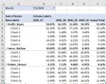
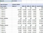
I am trying to summarize employee time sheet data using a pivot table. I want it to break down by employee the percentage of time they are spending on each client each week. I have been able to do that. Ideally, I would then be able to show in the table a summary for each employee of the total hours billed during the week (so absolute total, not the percentages that are used in the body of the table). Anyone know if this is doable? Photo attached. Each column represents a week. I would want rows 5, 11, and 15 to show the total hours that employee spent across all clients for the week. Thanks!

 

[OceanStateSixSpeed]

It's impossible to answer this without seeing how you structured your input data.
If your source data is in hours, you just have to undo the "show as percent" setting you did in order to show it as a percent.
If your source data is in percents, then you'll need to add a new column or columns, or you could use the calculated field.

 

[xtapalat]

Thanks. Have attached a screenshot that gives a sense of the raw data structure. Data source is in hours. The problem I am having is that, when I try to undo the 'show values as percent of parent row total' selection, even if I just do it for a row with the parents in it, it makes the change for the entire pivot table. What I am trying to get is output like the attached screenshot which reports the actual sum in the parent and then shows the percent breakdown below (so combination of both percent and actual reporting in the pivot table).

 

[OceanStateSixSpeed]

Ah ok. I don't know an "easy" way to fix this, but you can create your own custom table based on the pivot, but this takes some effort to set up.

Start by making a pivot with the columns in tabular form. Then use the GetPivotData function to mirror the data in another table, see my quick and dirty example below.

After that you can add whatever rows you want. For exmple, add a row between 6 and 7 for the summary for Jim, using SUMPRODUCT to get the sum. Then add 2 more columns to the right, where you convert the hours to % for everything except the subtotal rows you added. Then you can just hide the columns you no longer need (I and J in my exmple)

It takes a while to set up and it's not the most elegant, but once it's set up it will work.

 

[OceanStateSixSpeed]

...Something like this

 

[OceanStateSixSpeed]

Then clean it up a bit and it looks like this:

 

[xtapalat]

That's great. Didn't know you could do that. Thanks so much!