Placing coordinates to which grid it belongs (Combining IF with HLOOKUP or Index Match)

mvbarus

New Member
Joined
Jul 13, 2021
Messages
5
Office Version
  1. 365
  2. 2019
Platform
  1. Windows
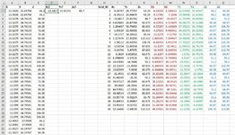
I have a set of data of coordinates X, Y, Z (Column A, B, C). They are located on a surface with grids consisting of 26 cells. I also have the information of those grids (Xc, Yc, Zc are the centre point of those grids, and X1 until Z2 are the corner points of them). (See attachment)

For each point, I want the columns D, E, F to return the value of Xc, Yc, Zc of the grid to which that point belongs to.
In other words, D2 will search in column I horizontally where the value of A2 is between X1 and X2, B2 is between Y1 and Y2, and C3 is between Z1 and Z2.

I tried writing the function below where it must fulfil those 3 conditions.
Excel Formula:
=IF(AND(A3>=MIN($L$4,$M$4),A3<=MAX($L$4,$M$4),
B3>=MIN($N$4,$O$4),B3<=MAX($N$4,$O$4),
C3>=MIN($P$4,$Q$4),C3<=MAX($P$4,$Q$4)),$I$4,0)

Here the function search only in Grid number 3 (because I manually know it belongs there). Therefore, it didn't search the set of Grid data. I know I should use either Hlookup or Index Match, but I just couldn't figure out where and how to put them.

Please help.
 

Attachments

  • Screenshot 2021-07-13 193520-min.jpg
    Screenshot 2021-07-13 193520-min.jpg
    218.3 KB · Views: 19

Excel Facts

Who is Mr Spreadsheet?
Author John Walkenbach was Mr Spreadsheet until his retirement in June 2019.
Welcome to Mr Excel Forum

If there is only one grid that meets the conditions I think SUMIFS should work, for example

Formula in D2 (to get Xc)
=SUMIFS(I$2:I$27,L$2:L$27,"<="&A2,M$2:M$27,">="&A2)

Try similar formulas to get Yc and Zc, adjusting the ranges

Hope this helps

M.
 
Upvote 0
Looking more carefully at your data i noticed there are identical values (pairs) in column Z, for example P2-Q2 and P3-Q3.
In this case SUMIFS doesn't work. We need a different formula

M.
 
Upvote 0
A picture is not helpful - it's not possible copy/paste for testing purpose

To post your data try

M.
 
Upvote 0
A picture is not helpful - it's not possible copy/paste for testing purpose

To post your data try

M.
So sorry. Below is the Mini-Sheet.

Book5.xlsx
ABCDEFGHIJKLMNOPQ
1XYZXc?Yc?Zc?Grid_IDXcYcZcX1X2Y1Y2Z1Z2
2-13.582615.6970446.2-13.481715.8173148.71-0.3874728.7779753.29-6.015565.24061522.0706835.4852746.260.38
3-13.582615.6970450.22-8.1911220.6447553.29-9.17763-7.204619.4690621.8204346.260.38
4-13.127914.7613360.383-13.481715.8173148.7-16.9097-10.053711.7319919.9026246.251.2
5-13.127914.7613364.3840.61948326.4776462.675-4.276535.51549920.6427932.3124860.3864.97
6-13.127914.7613368.3852.28400730.7949385.855-0.572875.14088927.3902334.1996364.97106.74
7-13.127914.7613372.386-1.9352623.4330185.855-4.276530.40601120.6427926.2232364.97106.74
8-13.127914.7613376.387-10.172718.2832285.56-13.1279-7.2174514.7613321.8051160.38110.74
9-13.127914.7613380.3885.22747627.30206110.3152.8650057.58994724.4865830.11754106.74113.89
10-13.127914.7613384.3891.5811220.62292108.74-0.829333.99157417.7502523.49558106.74110.74
11-13.127914.7613388.3810-12.035413.8635487.855-13.1297-10.941112.9453214.7817664.97110.74
12-13.127914.7613392.3811-2.347965.4737587.855-10.94256.246554-1.7379112.6854164.97110.74
13-13.127914.7613396.3812-3.38246.60283262.675-13.12976.364864-1.576114.7817660.3864.97
14-13.127914.76133100.38138.356008-3.3712155.26.9813329.730683-4.5247-2.2177251.259.2
15-13.127914.76133104.381424.47085-16.768855.29.83097739.11073-29.0531-4.4845151.259.2
16-13.127914.76133108.381522.21419-11.850487.8556.24655438.18183-21.9628-1.7379164.97110.74
17-13.09914.7958160.381615.02999-7.063862.6756.36486423.69511-12.5515-1.576160.3864.97
18-13.09914.7958164.381731.4931-17.490162.67524.8539838.13223-21.6947-13.285460.3864.97
19-13.09914.7958168.381841.68349-25.9155.239.0409944.32599-29.0592-22.760851.259.2
20-13.09914.7958172.381939.47327-20.096562.67538.1322340.8143-21.6947-18.498360.3864.97
21-13.09914.7958176.382039.5669-20.296187.85538.1662940.96751-21.9652-18.626964.97110.74
22-13.09914.7958180.382146.97001-17.593658.08544.6239149.3161-20.3896-14.797651.264.97
23-13.09914.7958184.382246.96519-17.599385.85544.6239149.30646-20.3896-14.809164.97106.74
24-13.09914.7958188.382355.95778-9.0115455.7951.2964460.61913-14.5667-3.4563651.260.38
25-13.09914.7958192.382455.80033-8.8886762.67551.2627360.33792-14.2964-3.4809760.3864.97
26-13.09914.7958196.382555.95353-9.0172285.85551.2873860.61969-14.5781-3.4563264.97106.74
27-13.09914.79581100.382652.14406-7.64076110.31548.3741155.91401-12.1336-3.14791106.74113.89
28-13.09914.79581104.38
29-13.09914.79581108.38
30-12.406317.098946.2
31-12.406317.098950.2
32-11.922716.1976760.38
33-11.922716.1976764.38
34-11.922716.1976768.38
35-11.922716.1976772.38
Sheet1
Cell Formulas
RangeFormula
D2D2=IF(AND(A2>=MIN($L$4,$M$4),A2<=MAX($L$4,$M$4), B2>=MIN($N$4,$O$4),B2<=MAX($N$4,$O$4), C2>=MIN($P$4,$Q$4),C2<=MAX($P$4,$Q$4)),$I$4,0)
E2E2=IF(AND(A2>=MIN($L$4,$M$4),A2<=MAX($L$4,$M$4), B2>=MIN($N$4,$O$4),B2<=MAX($N$4,$O$4), C2>=MIN($P$4,$Q$4),C2<=MAX($P$4,$Q$4)),$J$4,0)
F2F2=IF(AND(A2>=MIN($L$4,$M$4),A2<=MAX($L$4,$M$4), B2>=MIN($N$4,$O$4),B2<=MAX($N$4,$O$4), C2>=MIN($P$4,$Q$4),C2<=MAX($P$4,$Q$4)),$K$4,0)
 
Upvote 0
Question
What is the expected result when more than one grid meet the conditions?

For example C2=46.2
Grids 1, 2 and 3 meet the conditions.

M.
 
Upvote 0
Question
What is the expected result when more than one grid meet the conditions?

For example C2=46.2
Grids 1, 2 and 3 meet the conditions.

M.
In that example, indeed C2 is between P and Q in all Grids 1 2 3, but the A2 and B2 coordinates didn't meet grid 1 and 2. Only grid 3 meet all condition (A2 is between L and M; B2 is between N and O; C2 is between P and Q.

However, there really are several points that belong to 2 grids, and I just need to pick one randomly. There are also several points that didn't belong to any grid, and this condition will return the value of 0.

Sorry if I made it more complicated :/
 
Upvote 0
Try

D2 copied down
=INDEX(I$2:I$27,AGGREGATE(15,6,(ROW(I$2:I$27)-ROW(I$2)+1)/((L$2:L$27<=A2)*(M$2:M$27>=A2)),1))

E2 copied down
=INDEX(J$2:J$27,AGGREGATE(15,6,(ROW(J$2:J$27)-ROW(J$2)+1)/((N$2:N$27<=B2)*(O$2:O$27>=B2)),1))

F2 copied down
=INDEX(K$2:K$27,AGGREGATE(15,6,(ROW(K$2:K$27)-ROW(K$2)+1)/((P$2:P$27<=C2)*(Q$2:Q$27>=C2)),1))

M.
Thank you for your suggestion.
But they only give the right Xc, Yc, Zc for the first point (row 2).
I copied them down and it somehow keeps repeating the same answer as row 2, except for Z but it also gives the wrong Zc.

However, I think you misunderstood something.
D2 will give a value in column I where the coordinates fulfil all 3 conditions:
1. A2 is between L and M
2. B2 is between N and O
3. C2 is between P and Q

E2 will give a value in column J also when A2, B2, C2 fulfil the same conditions.
The same applies when calculating F2.
 
Upvote 0

Forum statistics

Threads
1,215,020
Messages
6,122,709
Members
449,093
Latest member
Mnur

We've detected that you are using an adblocker.

We have a great community of people providing Excel help here, but the hosting costs are enormous. You can help keep this site running by allowing ads on MrExcel.com.
Allow Ads at MrExcel

Which adblocker are you using?

Disable AdBlock

Follow these easy steps to disable AdBlock

1)Click on the icon in the browser’s toolbar.
2)Click on the icon in the browser’s toolbar.
2)Click on the "Pause on this site" option.
Go back

Disable AdBlock Plus

Follow these easy steps to disable AdBlock Plus

1)Click on the icon in the browser’s toolbar.
2)Click on the toggle to disable it for "mrexcel.com".
Go back

Disable uBlock Origin

Follow these easy steps to disable uBlock Origin

1)Click on the icon in the browser’s toolbar.
2)Click on the "Power" button.
3)Click on the "Refresh" button.
Go back

Disable uBlock

Follow these easy steps to disable uBlock

1)Click on the icon in the browser’s toolbar.
2)Click on the "Power" button.
3)Click on the "Refresh" button.
Go back
Back
Top