Post COVID branch rostering

ashoksoft

New Member
Joined
Jul 19, 2009
Messages
6
Dear team,

I am faced with a unique situation and would really seek help here.. I work with an organization that has about 5000 staff members, who are working out of 159 branches. Each branch has a different seating capacity - now some branches have traditionally had more employees than the seating capacity. The post lockdown norms enforce physical distancing - due to which we are allowed to have 50% staffing of the total seats in the branch.

The new norms have 3 shift codes - WFF (Work from Field), WFO (Work from office) and WFH (Work from home).. while there is no restriction to the number of people who can be on WFH / WFF, you can only have 50% of the available seat count allowed to WFO. Employees who are on WFH / WFF may have to come to the office anywhere between 1 to 5 days in a week.

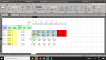
Now to tackle this I have created 3 rows above the data detailing Date, Week No. and Day. The rule is that for each branch code there is a restriction on the number of seats available. The total number of employees on WFO cannot exceed the seating limit per day, and cannot exceed the number of days in office per week. (The image below is a overly simplified view of the process) .. WO stands for week off.

I tried to write a formula ignoring circular references - but could not get the randomization of the days in the week possible. attaching a copy of the dummy sheet I made here - any help will be deeply appreciated.


1592278043560.png


Book4
ABCDEFGHIJKLMN
1Day : MonTueWedThuFriSatSun
2Week No.25252525252525
3Date :15-Jun16-Jun17-Jun18-Jun19-Jun20-Jun21-Jun
4Emp. IdEmployee NameBranch CodeSeats AvailableEmployees rostered in the branchPrimary RoleDays in office
510000Emp 1AHM00324WFH1WFHWFHWFOWFHWFHWOWO
610001Emp 2AHM00324WFH2WFOWFHWFHWFHWFOWOWO
710002Emp 3AHM00324WFF3WFFWFOWFOWFOWFHWOWO
810003Emp 4AHM00324WFH3WFOWFOWFHWFOWFHWOWO
910004Emp 5AHM00434WFH1
1010005Emp 6AHM00434WFF3
1110006Emp 7AHM00434WFH2
1210007Emp 8AHM00434WFH2
Sheet1
Cells with Conditional Formatting
CellConditionCell FormatStop If True
H5:N8Cell Value="WO"textNO
H5:N8Cell Value="WFF"textNO
H5:N8Cell Value="WFO"textNO
H5:N8Cell Value="WFH"textNO
 

Excel Facts

Lock one reference in a formula
Need 1 part of a formula to always point to the same range? use $ signs: $V$2:$Z$99 will always point to V2:Z99, even after copying
Whew... this seems to do it... I added a couple people to test it.
If you want to rotate the schedule then you should reorder the employees for subsequent weeks
Book2
BCDEFGHIJKLMN
1
2Day :MonTueWedThuFriSatSun
3Week No.25252525252525
4Date :15-Jun16-Jun17-Jun18-Jun19-Jun20-Jun21-Jun
5Employee NameBranch CodeSeats AvailableEmployees rostered in the branchPrimary RoleDays in office
6Emp 1AHM00324WFH1WFHWFHWFOWFHWFHWOWO
7Emp 2AHM00324WFH2WFOWFHWFHWFHWFOWOWO
8Emp 3AHM00324WFF3WFFWFOWFOWFOWFHWOWO
9Emp 4AHM00324WFH3WFOWFOWFHWFOWFHWOWO
10Emp 5AHM00434WFH1WFOWFHWFHWFHWFH
11Emp 6AHM00434WFF3WFFWFOWFOWFOWFF
12Emp 7AHM00434WFH2WFOWFHWFHWFHWFO
13Emp 8AHM00434WFH2WFHWFOWFOWFHWFH
14Emp 9AHM00434WFH2WFHWFHWFHWFOWFO
15Emp 10AHM00434WFH3WFOWFOWFOWFHWFH
Sheet1
Cell Formulas
RangeFormula
H10:L15H10=IF(COUNTIF($C$6:$C10,$C10)=1,IF(COLUMNS($H10:H10)<=$G10,"WFO",$F10),CHOOSE(IF(MATCH("WFO",$H9:$L9,0)+$G9>5,1,IF(MATCH("WFO",$H9:$L9,0)+$G9+$G10-1>5,2,3)),IF(OR(COLUMNS($H10:H10)<=MATCH("WFO",$H9:$L9,0)+$G9+$G10-1-5,COLUMNS($H10:H10)>=MATCH("WFO",$H9:$L9,0)+$G9),"WFO",$F10),IF(OR(COLUMNS($H10:H10)<=MATCH("WFO",$H9:$L9,0)+$G9+$G10-1-5,COLUMNS($H10:H10)>=MATCH("WFO",$H9:$L9,0)+$G9),"WFO",$F10),IF(AND(COLUMNS($H10:H10)<=MATCH("WFO",$H9:$L9,0)+$G9+$G10-1-IF($H9="WFO",COUNTIF(OFFSET($G9,0,1,1,$G9),"<>WFO"),0),COLUMNS($H10:H10)>=MATCH("WFO",$H9:$L9,0)+$G9+IF(AND(COLUMNS($H10:H10)>1,$G9>COLUMNS($H10:H10)-1),$G9-COLUMNS($H10:H10)-1,0)),"WFO",$F10)))


Hope this works for you
 
Upvote 0
Whew... this seems to do it... I added a couple people to test it.
If you want to rotate the schedule then you should reorder the employees for subsequent weeks
Book2
BCDEFGHIJKLMN
1
2Day :MonTueWedThuFriSatSun
3Week No.25252525252525
4Date :15-Jun16-Jun17-Jun18-Jun19-Jun20-Jun21-Jun
5Employee NameBranch CodeSeats AvailableEmployees rostered in the branchPrimary RoleDays in office
6Emp 1AHM00324WFH1WFHWFHWFOWFHWFHWOWO
7Emp 2AHM00324WFH2WFOWFHWFHWFHWFOWOWO
8Emp 3AHM00324WFF3WFFWFOWFOWFOWFHWOWO
9Emp 4AHM00324WFH3WFOWFOWFHWFOWFHWOWO
10Emp 5AHM00434WFH1WFOWFHWFHWFHWFH
11Emp 6AHM00434WFF3WFFWFOWFOWFOWFF
12Emp 7AHM00434WFH2WFOWFHWFHWFHWFO
13Emp 8AHM00434WFH2WFHWFOWFOWFHWFH
14Emp 9AHM00434WFH2WFHWFHWFHWFOWFO
15Emp 10AHM00434WFH3WFOWFOWFOWFHWFH
Sheet1
Cell Formulas
RangeFormula
H10:L15H10=IF(COUNTIF($C$6:$C10,$C10)=1,IF(COLUMNS($H10:H10)<=$G10,"WFO",$F10),CHOOSE(IF(MATCH("WFO",$H9:$L9,0)+$G9>5,1,IF(MATCH("WFO",$H9:$L9,0)+$G9+$G10-1>5,2,3)),IF(OR(COLUMNS($H10:H10)<=MATCH("WFO",$H9:$L9,0)+$G9+$G10-1-5,COLUMNS($H10:H10)>=MATCH("WFO",$H9:$L9,0)+$G9),"WFO",$F10),IF(OR(COLUMNS($H10:H10)<=MATCH("WFO",$H9:$L9,0)+$G9+$G10-1-5,COLUMNS($H10:H10)>=MATCH("WFO",$H9:$L9,0)+$G9),"WFO",$F10),IF(AND(COLUMNS($H10:H10)<=MATCH("WFO",$H9:$L9,0)+$G9+$G10-1-IF($H9="WFO",COUNTIF(OFFSET($G9,0,1,1,$G9),"<>WFO"),0),COLUMNS($H10:H10)>=MATCH("WFO",$H9:$L9,0)+$G9+IF(AND(COLUMNS($H10:H10)>1,$G9>COLUMNS($H10:H10)-1),$G9-COLUMNS($H10:H10)-1,0)),"WFO",$F10)))


Hope this works for you


I did try that - but after enabling iterative calculations also on - I seem to be getting all WFO on the 10th row - and #Value! in the next row :( What you have shown in the example is exactly what I am looking out for.
 

Attachments

  • 1592383681347.png
    1592383681347.png
    142.6 KB · Views: 2
Upvote 0
My formula starts in cell H10 as your original post did. Your image starts in G10.
Insert a column in your sheet at beginning before pasting my formula for apples to apples.
Then delete your added column and that should fix it.
 
Upvote 0
Works like a charm!!! Thanks a zillion. My bad - missed the Coloumn :)


My formula starts in cell H10 as your original post did. Your image starts in G10.
Insert a column in your sheet at beginning before pasting my formula for apples to apples.
Then delete your added column and that should fix it.
 
Upvote 0
So glad to hear that... I didnt want to have to take another crack at that one.
 
Upvote 0
Thanks bud :)

Ran into a little deep water there - tried it on the actual large data set but it seems to have gone awry there. Originally the branch codes were all jumbled -sorted it in an order but guess its going wrong somewhere.

Uncertain of the forum rules here - am I allowed to share a link with the excel book ? anyway here's what I got :)


Day :MonTueWedThuFriSatSun
Week No.
25​
25​
25​
25​
25​
25​
25​
Date :
Emp IdEmployee NameBranch CodeSeats AvailableEmployees rostered in the branchPrimary RoleDays in office6/15/20206/16/20206/17/20206/18/20206/19/20206/20/20206/21/2020
100000Emp 001AGR00127
69​
WFF
2​
WFOWFOWFFWFFWFF
100001Emp 002AGR00127
69​
WFH
1​
WFHWFOWFOWFHWFH
100002Emp 003AGR00127
69​
WFF
6​
WFOWFOWFOWFOWFO
100003Emp 004AGR00127
69​
WFH
3​
WFOWFOWFOWFOWFH
100004Emp 005AGR00127
69​
WFF
6​
WFOWFOWFOWFOWFO
100005Emp 006AGR00127
69​
WFF
6​
WFOWFOWFOWFOWFO
100006Emp 007AGR00127
69​
WFF
6​
WFOWFOWFOWFOWFO
100007Emp 008AGR00127
69​
WFF
6​
WFOWFOWFOWFOWFO
100008Emp 009AGR00127
69​
WFF
6​
WFOWFOWFOWFOWFO
100009Emp 010AGR00127
69​
WFH
3​
WFOWFOWFOWFOWFH
100010Emp 011AGR00127
69​
WFH
1​
WFHWFHWFOWFOWFH
100011Emp 012AGR00127
69​
WFF
6​
WFOWFOWFOWFOWFO
100012Emp 013AGR00127
69​
WFH
2​
WFOWFOWFOWFHWFH
100013Emp 014AGR00127
69​
WFH
1​
WFHWFOWFOWFHWFH
100014Emp 015AGR00127
69​
WFF
6​
WFOWFOWFOWFOWFO
100015Emp 016AGR00127
69​
WFF
6​
WFOWFOWFOWFOWFO
100016Emp 017AGR00127
69​
WFF
6​
WFOWFOWFOWFOWFO
100017Emp 018AGR00127
69​
WFF
6​
WFOWFOWFOWFOWFO
100018Emp 019AGR00127
69​
WFH
2​
WFOWFOWFOWFHWFH
100019Emp 020AGR00127
69​
WFH
2​
WFHWFOWFOWFOWFH
100020Emp 021AGR00127
69​
WFF
6​
WFOWFOWFOWFOWFO
100021Emp 022AGR00127
69​
WFF
6​
WFOWFOWFOWFOWFO
100022Emp 023AGR00127
69​
WFO
3​
WFOWFOWFOWFOWFO
100023Emp 024AGR00127
69​
WFF
6​
WFOWFOWFOWFOWFO
100024Emp 025AGR00127
69​
WFH
2​
WFOWFOWFOWFHWFH
100025Emp 026AGR00127
69​
WFF
6​
WFOWFOWFOWFOWFO
100026Emp 027AGR00127
69​
WFF
6​
WFOWFOWFOWFOWFO
100027Emp 028AGR00127
69​
WFF
6​
WFOWFOWFOWFOWFO
100028Emp 029AGR00127
69​
WFF
6​
WFOWFOWFOWFOWFO
100029Emp 030AGR00127
69​
WFH
3​
WFOWFOWFOWFOWFH
100030Emp 031AGR00127
69​
WFO
3​
WFOWFOWFOWFOWFO
100031Emp 032AGR00127
69​
WFH
3​
WFOWFHWFHWFOWFO
100032Emp 033AGR00127
69​
WFH
2​
WFHWFHWFOWFHWFH
100033Emp 034AGR00127
69​
WFH
2​
WFOWFHWFHWFHWFO
100034Emp 035AGR00127
69​
WFF
6​
WFOWFOWFOWFOWFO
100035Emp 036AGR00127
69​
WFH
2​
WFOWFOWFOWFHWFH
100036Emp 037AGR00127
69​
WFH
1​
WFHWFOWFOWFHWFH
100037Emp 038AGR00127
69​
WFF
6​
WFOWFOWFOWFOWFO
100038Emp 039AGR00127
69​
WFH
1​
WFOWFOWFHWFHWFH
100039Emp 040AHM00213
114​
WFF
6​
WFOWFOWFOWFOWFO
100040Emp 041AHM00213
114​
WFF
6​
WFOWFOWFOWFOWFO
100041Emp 042AHM00213
114​
WFF
6​
WFOWFOWFOWFOWFO
100042Emp 043AHM00213
114​
WFF
6​
WFOWFOWFOWFOWFO
100043Emp 044AHM00213
114​
WFH
1​
WFOWFOWFHWFHWFH
100044Emp 045AHM00213
114​
WFF
6​
WFOWFOWFOWFOWFO
100045Emp 046AHM00213
114​
WFF
6​
WFOWFOWFOWFOWFO
100046Emp 047AHM00213
114​
WFH
2​
WFOWFOWFOWFHWFH
100047Emp 048AHM00213
114​
WFF
6​
WFOWFOWFOWFOWFO
100048Emp 049AHM00213
114​
WFH
3​
WFOWFOWFOWFOWFH
100049Emp 050AHM00213
114​
WFF
6​
WFOWFOWFOWFOWFO
100050Emp 051AHM00352
295​
WFH
1​
WFOWFHWFHWFHWFH
100051Emp 052AHM00352
295​
WFH
2​
WFHWFOWFOWFHWFH
100052Emp 053AHM00352
295​
WFF
6​
WFOWFOWFOWFOWFO
100053Emp 054AHM00352
295​
WFH
3​
WFOWFOWFOWFOWFH
100054Emp 055AHM00352
295​
WFH
1​
WFHWFHWFOWFOWFH
100055Emp 056AHM00352
295​
WFF
6​
WFOWFOWFOWFOWFO
100056Emp 057AHM00352
295​
WFH
2​
WFOWFOWFOWFHWFH
100057Emp 058AHM00352
295​
WFH
2​
WFHWFOWFOWFOWFH
100058Emp 059AHM00352
295​
WFF
6​
WFOWFOWFOWFOWFO
100059Emp 060AHM00352
295​
WFH
3​
WFOWFOWFOWFOWFH
100060Emp 061AHM00352
295​
WFH
2​
WFHWFHWFOWFOWFO
100061Emp 062AHM00352
295​
WFF
6​
WFOWFOWFOWFOWFO
100062Emp 063AHM00352
295​
WFF
6​
WFOWFOWFOWFOWFO
100063Emp 064AHM00352
295​
WFH
1​
WFOWFOWFHWFHWFH
100064Emp 065AHM00352
295​
WFF
6​
WFOWFOWFOWFOWFO
100065Emp 066AHM00352
295​
WFH
3​
WFOWFOWFOWFOWFH
100066Emp 067AHM00352
295​
WFH
1​
WFHWFHWFOWFOWFH
100067Emp 068AHM00352
295​
WFH
1​
WFHWFHWFHWFOWFH
100068Emp 069AHM00352
295​
WFH
3​
WFOWFOWFHWFHWFO
100069Emp 070AHM00352
295​
WFH
3​
WFOWFHWFHWFOWFO
100070Emp 071AHM00352
295​
WFF
6​
WFOWFOWFOWFOWFO
100071Emp 072AHM00352
295​
WFH
2​
WFOWFOWFOWFHWFH
100072Emp 073AHM00352
295​
WFH
2​
WFHWFOWFOWFOWFH
100073Emp 074AHM00352
295​
WFH
1​
WFHWFHWFHWFOWFH
100074Emp 075AHM00352
295​
WFH
1​
WFHWFHWFHWFHWFO
100075Emp 076AHM00352
295​
WFH
2​
WFOWFOWFHWFHWFH
100076Emp 077AHM00352
295​
WFH
1​
WFHWFOWFOWFHWFH
100077Emp 078AHM00352
295​
WFH
1​
WFHWFHWFOWFHWFH
100078Emp 079AHM00352
295​
WFF
6​
WFOWFOWFOWFOWFO
100079Emp 080AHM00352
295​
WFH
1​
WFOWFOWFHWFHWFH
100080Emp 081AHM00352
295​
WFF
6​
WFOWFOWFOWFOWFO
100081Emp 082AHM00352
295​
WFH
1​
WFOWFOWFHWFHWFH
100082Emp 083AHM00352
295​
WFH
1​
WFHWFOWFHWFHWFH
100083Emp 084AHM00352
295​
WFF
6​
WFOWFOWFOWFOWFO
100084Emp 085AHM00352
295​
WFF
6​
WFOWFOWFOWFOWFO
100085Emp 086AHM00352
295​
WFH
3​
WFOWFOWFOWFOWFH
100086Emp 087AHM00352
295​
WFH
3​
WFOWFHWFHWFOWFO
100087Emp 088AHM00352
295​
WFO
3​
WFOWFOWFOWFOWFO
100088Emp 089AHM00352
295​
WFH
1​
WFHWFHWFOWFOWFH
100089Emp 090AHM00352
295​
WFH
3​
WFOWFHWFHWFOWFO
100090Emp 091AHM00352
295​
WFH
1​
WFHWFHWFHWFHWFH
100091Emp 092AHM00352
295​
WFF
6​
#N/A​
#N/A​
#N/A​
#N/A​
#N/A​
100092Emp 093AHM00352
295​
WFH
1​
#N/A​
#N/A​
#N/A​
#N/A​
#N/A​
100093Emp 094AHM00352
295​
WFF
6​
#N/A​
#N/A​
#N/A​
#N/A​
#N/A​
100094Emp 095AHM00352
295​
WFH
3​
#N/A​
#N/A​
#N/A​
#N/A​
#N/A​
100095Emp 096AHM00352
295​
WFH
1​
#N/A​
#N/A​
#N/A​
#N/A​
#N/A​
100096Emp 097AHM00352
295​
WFH
3​
#N/A​
#N/A​
#N/A​
#N/A​
#N/A​
100097Emp 098AHM00352
295​
WFH
1​
#N/A​
#N/A​
#N/A​
#N/A​
#N/A​
100098Emp 099AHM00352
295​
WFH
1​
#N/A​
#N/A​
#N/A​
#N/A​
#N/A​
100099Emp 100AHM00352
295​
WFH
1​
#N/A​
#N/A​
#N/A​
#N/A​
#N/A​
100100Emp 101AHM00352
295​
WFH
1​
#N/A​
#N/A​
#N/A​
#N/A​
#N/A​
100101Emp 102AHM00352
295​
WFH
3​
#N/A​
#N/A​
#N/A​
#N/A​
#N/A​
100102Emp 103AHM00352
295​
WFH
1​
#N/A​
#N/A​
#N/A​
#N/A​
#N/A​
100103Emp 104AHM00352
295​
WFH
1​
#N/A​
#N/A​
#N/A​
#N/A​
#N/A​
100104Emp 105AHM00352
295​
WFF
6​
#N/A​
#N/A​
#N/A​
#N/A​
#N/A​
100105Emp 106AHM00352
295​
WFH
3​
#N/A​
#N/A​
#N/A​
#N/A​
#N/A​
100106Emp 107AHM00352
295​
WFH
2​
#N/A​
#N/A​
#N/A​
#N/A​
#N/A​
100107Emp 108AHM00352
295​
WFH
2​
#N/A​
#N/A​
#N/A​
#N/A​
#N/A​
100108Emp 109AHM00352
295​
WFH
3​
#N/A​
#N/A​
#N/A​
#N/A​
#N/A​
100109Emp 110AHM00352
295​
WFF
6​
#N/A​
#N/A​
#N/A​
#N/A​
#N/A​
100110Emp 111AHM00352
295​
WFH
2​
#N/A​
#N/A​
#N/A​
#N/A​
#N/A​
 
Upvote 0
My formula starts in cell H10 as your original post did. Your image starts in G10.
Insert a column in your sheet at beginning before pasting my formula for apples to apples.
Then delete your added column and that should fix it.
Oops the xl2bb did not get the formulas.. apparently the xl2bb thing cannot post the content - says too much data ...

Google Drive link

I have uploaded the excel file here - in case you can help me on this
 
Upvote 0
Noooooooo!!!!!
Ok... here we go.
I sorted your list by location ascending and then number of days in office descending.
Otherwise, everytime you have a 5 day person, the next person will start on a Monday... you will have overcrowded Mondays and ghosttown fridays.
The sorting gives yoiu a true cascade,
I also changed each of your people allowed 6 days to 5, as you cannot have 6 days in a 5 day week... it will break things
Also, you have a number of people who had WFO as their option when not WFO... I changed them to WTF... you need a second option or bad math
Here is the adjusted and to my knowledge working code... I also ran into the too much data link so I am abbreviating it... but it works for me.

Book1
ABCDEFGHIJKL
2Day :MonTueWedThuFri
3Week No.2525252525
4Date :
5Emp IdEmployee NameBranch CodeSeats AvailableEmployees rostered in the branchPrimary RoleDays in office6/15/20206/16/20206/17/20206/18/20206/19/2020
6100002Emp 003AGR0012769WFF5WFOWFOWFOWFOWFO
7100003Emp 004AGR0012769WFH3WFOWFOWFOWFHWFH
8100009Emp 010AGR0012769WFH3WFOWFHWFHWFOWFO
9100022Emp 023AGR0012769WTF3WTFWFOWFOWFOWTF
10100033Emp 034AGR0012769WFH2WFOWFHWFHWFHWFO
11100035Emp 036AGR0012769WFH2WFHWFOWFOWFHWFH
12100001Emp 002AGR0012769WFH1WFHWFHWFHWFOWFH
13100010Emp 011AGR0012769WFH1WFHWFHWFHWFHWFO
14100013Emp 014AGR0012769WFH1WFOWFHWFHWFHWFH
15100040Emp 041AHM00213114WFF5WFOWFOWFOWFOWFO
16100041Emp 042AHM00213114WFF5WFOWFOWFOWFOWFO
Sheet1
Cell Formulas
RangeFormula
H6:L16H6=IF(COUNTIF($C$6:$C6,$C6)=1,IF(COLUMNS($H6:H6)<=$G6,"WFO",$F6),CHOOSE(IF(MATCH("WFO",$H5:$L5,0)+$G5>5,1,IF(MATCH("WFO",$H5:$L5,0)+$G5+$G6-1-IF($H5="WFO",COUNTIF(OFFSET($G5,0,1,1,$G5),"<>WFO"),0)>5,2,3)),IF(OR(COLUMNS($H6:H6)<=MATCH("WFO",$H5:$L5,0)+$G5+$G6-1-5,COLUMNS($H6:H6)>=MATCH("WFO",$H5:$L5,0)+$G5),"WFO",$F6),IF(OR(COLUMNS($H6:H6)<=MATCH("WFO",$H5:$L5,0)+$G5+$G6-1-5,COLUMNS($H6:H6)>=MATCH("WFO",$H5:$L5,0)+$G5),"WFO",$F6),IF(AND(COLUMNS($H6:H6)<=MATCH("WFO",$H5:$L5,0)+$G5+$G6-1-IF($H5="WFO",COUNTIF(OFFSET($G5,0,1,1,$G5),"<>WFO"),0),COLUMNS($H6:H6)>=MATCH("WFO",$H5:$L5,0)+$G5-IF($H5="WFO",COUNTIF(OFFSET($G5,0,1,1,$G5),"<>WFO"),0)),"WFO",$F6)))
 
Upvote 0
Thanks a ton, will try this. The reason you saw a few 6 day working cases is cos some depts work on Saturdays also.. they are automatically WFO on their working Saturdays (and that's to be ignored in our 5 day week calculation. )

I'll try this with days working descending and confirm shortly. Thanks a zillion buddy.
 
Upvote 0

Forum statistics

Threads
1,215,019
Messages
6,122,707
Members
449,093
Latest member
Mnur

We've detected that you are using an adblocker.

We have a great community of people providing Excel help here, but the hosting costs are enormous. You can help keep this site running by allowing ads on MrExcel.com.
Allow Ads at MrExcel

Which adblocker are you using?

Disable AdBlock

Follow these easy steps to disable AdBlock

1)Click on the icon in the browser’s toolbar.
2)Click on the icon in the browser’s toolbar.
2)Click on the "Pause on this site" option.
Go back

Disable AdBlock Plus

Follow these easy steps to disable AdBlock Plus

1)Click on the icon in the browser’s toolbar.
2)Click on the toggle to disable it for "mrexcel.com".
Go back

Disable uBlock Origin

Follow these easy steps to disable uBlock Origin

1)Click on the icon in the browser’s toolbar.
2)Click on the "Power" button.
3)Click on the "Refresh" button.
Go back

Disable uBlock

Follow these easy steps to disable uBlock

1)Click on the icon in the browser’s toolbar.
2)Click on the "Power" button.
3)Click on the "Refresh" button.
Go back
Back
Top