Press a cell and then create cells with specific formula

[Unexpc]

Hi guys
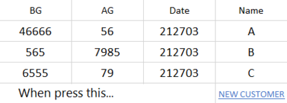
i have sheet that just list of customers, i insert costumers name in one column and other data i want to have in next columns
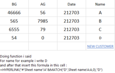
for name of customers of have this formula : =HYPERLINK("#'Sheet name'!A"&MATCH("Name of Customer",Sheet name!A:A,0),"Name of Customer")
sheet name that is sheet customer that belong data in it, for example for me Work for sheet name
another formula this is in next columns
=IFERROR(INDEX(Sheet name!B:B,MATCH($I4,Sheet name!A:A,0)-2,0),"")
=IFERROR(SUM(INDEX(Sheet name!D:D,MATCH($I3,Sheet name!A:A,0)+1,0):INDEX(Sheet name!E:E,MATCH($I4,Sheet name!A:A,0)-2,0)),"")
=IFERROR(SUM(INDEX(Sheet name!F:F,MATCH($I3,Sheet name!A:A,0)+1,0):INDEX(Sheet name!G:G,MATCH($I4,Sheet name!A:A,0)-2,0)),"")
this 3 formulas drag and fill in next rows
now
i want when select cell after last customer that may write NEW CUSTOMER, create a new first formula with the name that i write and then drag and fill this 3 formulas in that row and still stay this cell NEW CUSTOMER after that...

 

[maabadi]

It isn't problem at all. for e.g.

Lr3 = Sheets("Work").Range("A" & Rows.Count).End(xlUp).Row - 9

But I think for you it is better use my last code & you don't tell what is your problems with my last code.

 

[Unexpc]

It isn't problem at all. for e.g.

Lr3 = Sheets("Work").Range("A" & Rows.Count).End(xlUp).Row - 9

But I think for you it is better use my last code & you don't tell what is your problems with my last code.

before i select new customer last formula of last customer :
=IFERROR(INDEX(Work!B:B,MATCH($I14,Work!A:A,0)-2,0),"")
when i select new customer after this things happened:
first this formula convert to this (wrong order for column J) :
=IFERROR(INDEX(Work!B:B,MATCH($I15,Work!A:A,0)-2,0),"")
but for formula of columns K and L have correct order
and for new customer added, wrong give hyperlink of data of previous customer of this (not give a name of colored cell)
about formula of new customer Columns K and L is have correct order and formula of column J this is:
=IFERROR(INDEX(Work!B:B,MATCH($I16,Work!A:A,0)-2,0),"")
for before cell is correct order but in generally have wrong order

 

[maabadi]

Because you gave wrong source for match formula. I check your first formula for Customer A at column I (row 3 = Cell I3)
But Your match section search for I4 means search for Customer B & when We Insert Cell then formula changes to one row more.
Then I think your first formula should be =IFERROR(INDEX(Work!B:B,MATCH($I3,Work!A:A,0)-2,0),"")

But if your formula give correct result. Only main two first customer and clear others. Then Try this code:

Private Sub Worksheet_SelectionChange(ByVal Target As Range)
Dim i As Long, j As Long, Lr1 As Long, Lr2 As Long, Cr1 As Long, Cr1R As String, Cr2 As Long, Cr2R As String
Dim Lr3 As Long, Lr4 As Long
Lr1 = Range("I" & Rows.Count).End(xlUp).Row
Lr2 = Range("N" & Rows.Count).End(xlUp).Row
Lr3 = Sheets("Work").Range("A" & Rows.Count).End(xlUp).Row
Lr4 = Sheets("Paper").Range("A" & Rows.Count).End(xlUp).Row
'Lr5 = Sheets("Paper").Range("A" & Rows.Count).End(xlUp).Row
On Error Resume Next
 
  If Not Intersect(Target, Range("I" & Lr1)) Is Nothing Then
   If Target.Count = 1 Then
    Application.EnableEvents = False
     Range("I" & Lr1 & ":M" & Lr1).Insert Shift:=xlDown
     Range("I" & Lr1).Value = Sheets("Work").Range("A" & (Lr1 - 3) * 6 + 1).Value
     Cr1 = Application.WorksheetFunction.Match(Range("I" & Lr1).Value, Sheets("Work").Range("A1:A" & Lr3), 0)
     Cr1R = Range("A" & Cr1).Address
     Range("J" & Lr1 - 2 & ":L" & Lr1 - 2).AutoFill Destination:=Range("J" & Lr1 - 2 & ":L" & Lr1)
     Sheets("Dashboard").Hyperlinks.Add Anchor:=Range("I" & Lr1), Address:="", SubAddress:="'" & Sheets("Work").Name & "'!" & Cr1R, TextToDisplay:=Range("I" & Lr1).Value
    Application.EnableEvents = True
   End If
  End If
    If Not Intersect(Target, Range("N" & Lr2)) Is Nothing Then
   If Target.Count = 1 Then
    Application.EnableEvents = False
     Range("N" & Lr2 & ":Q" & Lr2).Insert Shift:=xlDown
     Range("N" & Lr2).Value = Sheets("Paper").Range("A" & (Lr2 - 3) * 6 + 1).Value
     Cr2 = Application.WorksheetFunction.Match(Range("N" & Lr2).Value, Sheets("Paper").Range("A1:A" & Lr4), 0)
     Cr2R = Range("A" & Cr2).Address
     Range("O" & Lr2 - 2 & ":Q" & Lr2 - 2).AutoFill Destination:=Range("O" & Lr2 - 2 & ":Q" & Lr2)
     Sheets("Dashboard").Hyperlinks.Add Anchor:=Range("N" & Lr2), Address:="", SubAddress:="'" & Sheets("Paper").Name & "'!" & Cr2R, TextToDisplay:=Range("N" & Lr2).Value
    Application.EnableEvents = True
   End If
  End If
End Sub

 

[Unexpc]

Because you gave wrong source for match formula. I check your first formula for Customer A at column I (row 3 = Cell I3)
But Your match section search for I4 means search for Customer B & when We Insert Cell then formula changes to one row more.
Then I think your first formula should be =IFERROR(INDEX(Work!B:B,MATCH($I3,Work!A:A,0)-2,0),"")

But if your formula give correct result. Only main two first customer and clear others. Then Try this code:

Private Sub Worksheet_SelectionChange(ByVal Target As Range)
Dim i As Long, j As Long, Lr1 As Long, Lr2 As Long, Cr1 As Long, Cr1R As String, Cr2 As Long, Cr2R As String
Dim Lr3 As Long, Lr4 As Long
Lr1 = Range("I" & Rows.Count).End(xlUp).Row
Lr2 = Range("N" & Rows.Count).End(xlUp).Row
Lr3 = Sheets("Work").Range("A" & Rows.Count).End(xlUp).Row
Lr4 = Sheets("Paper").Range("A" & Rows.Count).End(xlUp).Row
'Lr5 = Sheets("Paper").Range("A" & Rows.Count).End(xlUp).Row
On Error Resume Next

  If Not Intersect(Target, Range("I" & Lr1)) Is Nothing Then
   If Target.Count = 1 Then
    Application.EnableEvents = False
     Range("I" & Lr1 & ":M" & Lr1).Insert Shift:=xlDown
     Range("I" & Lr1).Value = Sheets("Work").Range("A" & (Lr1 - 3) * 6 + 1).Value
     Cr1 = Application.WorksheetFunction.Match(Range("I" & Lr1).Value, Sheets("Work").Range("A1:A" & Lr3), 0)
     Cr1R = Range("A" & Cr1).Address
     Range("J" & Lr1 - 2 & ":L" & Lr1 - 2).AutoFill Destination:=Range("J" & Lr1 - 2 & ":L" & Lr1)
     Sheets("Dashboard").Hyperlinks.Add Anchor:=Range("I" & Lr1), Address:="", SubAddress:="'" & Sheets("Work").Name & "'!" & Cr1R, TextToDisplay:=Range("I" & Lr1).Value
    Application.EnableEvents = True
   End If
  End If
    If Not Intersect(Target, Range("N" & Lr2)) Is Nothing Then
   If Target.Count = 1 Then
    Application.EnableEvents = False
     Range("N" & Lr2 & ":Q" & Lr2).Insert Shift:=xlDown
     Range("N" & Lr2).Value = Sheets("Paper").Range("A" & (Lr2 - 3) * 6 + 1).Value
     Cr2 = Application.WorksheetFunction.Match(Range("N" & Lr2).Value, Sheets("Paper").Range("A1:A" & Lr4), 0)
     Cr2R = Range("A" & Cr2).Address
     Range("O" & Lr2 - 2 & ":Q" & Lr2 - 2).AutoFill Destination:=Range("O" & Lr2 - 2 & ":Q" & Lr2)
     Sheets("Dashboard").Hyperlinks.Add Anchor:=Range("N" & Lr2), Address:="", SubAddress:="'" & Sheets("Paper").Name & "'!" & Cr2R, TextToDisplay:=Range("N" & Lr2).Value
    Application.EnableEvents = True
   End If
  End If
End Sub

i insert =IFERROR(INDEX(Work!B:B,MATCH($I4,Work!A:A,0)-2,0),"") because front of first customer is empty and data of first customer show front of second customer and next customer like this, that is column show data in wrong order
about this formula, please see this post SUM in changeable range between two texts
but for hyperlink still give wrong data, please explain what giving hyperlink you insert?

 

[maabadi]

but for hyperlink still give wrong data, please explain what giving hyperlink you insert?

I test it on your uploaded file. AND it work without problem
1. this line find match data at other sheet with Customer Name:

Cr1 = Application.WorksheetFunction.Match(Range("I" & Lr1).Value, Sheets("Work").Range("A1:A" & Lr3), 0)

2. this is Address of it

Cr1R = Range("A" & Cr1).Address

3. AND These line Add hyperlink to that cell:

Sheets("Dashboard").Hyperlinks.Add Anchor:=Range("N" & Lr2), Address:="", SubAddress:="'" & Sheets("Paper").Name & "'!" & Cr2R, TextToDisplay:=Range("N" & Lr2).Value

Anchor is the cell we add hyperlink to it
SubAddress is the address of matched value at other sheet to Anchor.

Book1.xlsm

 

[Unexpc]

I test it on your uploaded file. AND it work without problem
1. this line find match data at other sheet with Customer Name:

Cr1 = Application.WorksheetFunction.Match(Range("I" & Lr1).Value, Sheets("Work").Range("A1:A" & Lr3), 0)

2. this is Address of it

Cr1R = Range("A" & Cr1).Address

3. AND These line Add hyperlink to that cell:

Sheets("Dashboard").Hyperlinks.Add Anchor:=Range("N" & Lr2), Address:="", SubAddress:="'" & Sheets("Paper").Name & "'!" & Cr2R, TextToDisplay:=Range("N" & Lr2).Value

Anchor is the cell we add hyperlink to it
SubAddress is the address of matched value at other sheet to Anchor.

Book1.xlsm

i test file you upload, i think i have problem because i write data in column A and this column not just for customer name, because when i write any data in column A, function not doing correct after that, or if this not right, what am i do?

 

[maabadi]

Please upload image of dashboard sheet to I understand For which columns you want macro?

 

[maabadi]

If you say at Work and Sheet Paper at Column A have another data more than customer name, It's not problem.
We use match function to find correct customer name.

 

[Unexpc]

If you say at Work and Sheet Paper at Column A have another data more than customer name, It's not problem.
We use match function to find correct customer name.

yes, so no any problem, why giving wrong hyperlink for me?
that is no correct match to find and just give a data from a customer

 

[Unexpc]

Please upload image of dashboard sheet to I understand For which columns you want macro?

my example that i file uploaded but i say again maybe i can mean what am i want:
no consider all formula i say only what am i want in dashboard
i have two workbook, both of workbook have same data, different between two workbook, one of them for any customer have separate sheet, and other have two sheet that divide several customer that i named Work and Paper
dashboard for this two workbook have same format with different find data
for first the hyperlink is simple, just find sheet name and this insert in Column I, and next data i want find out, find last date of sheet and insert in column J and two next column, for column K in dashboard SUM of Column D:E of sheet for every customer and for Column L SUM of Ccolumn F:G for sheet for every customer, and continue in dashboard Column N:Q like before that
however this is not my first question, this is i ask you about second workbook
in Work and Paper, have several customer, in dashboard first hyperlink to specific text that written name of each customer and i colored a row for separate every customer, next column in dashboard find last date of a customer before next customer data (until that colored row) and in next two column of dashboard, both of column sum specific range between two customer, a point that when i want add data for any customer in this workbook i first insert row and after that fill with data, so range is changable
however, i make second workbook for prevent for many sheets in workbook, if you think this is not good, i thinking about that find a way when select name of every customer, sheet unhide and when select other sheet except that sheet, that sheet customer is hidden again
what is you suggestion?