Pulling loan # for specific employees into a different sheet.

[Cyndi2210]

Hi,

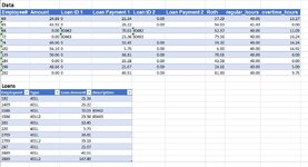
I am trying to show the value from the "Description" column from the "Loans" sheet into the "Data" sheet for the specific employee. Type 401L should populate Loan ID 1 and 401L2 should populate Loan ID 2. Any person without a loan should display as blank.

Thanks in advance for your help.

 

[awoohaw]

You're example does not have any related Employee ID's in the two tables.
Assuming that eventually you'll have an EmployeeID match.

Please update your profile and advise which version of excel you use. Also, the xl2bb add in (link below) is the best way to share your questions/data and best help the forum help you.

Book1
	A	B	C	D	E
1	Data
2	Emp#	Loan ID1	Loa ID2
3	60
4	65
5	66	80462
6	72		80463
7
8	Loans	Type		DESCR
9	102	401L
10	1409	401L
11	66	401L		80462
12	72	401L2		80463
13
Sheet1

Cell Formulas
Range	Formula
D9:D12	D9	=IFERROR(INDEX(INDEX($B$3:$C$6,MATCH(A9,$A$3:$A$6,0),0),MATCH(B9,{"401L","401L2",0})),"")

 

[Cyndi2210]

I am missing something because it didn't work. They are in separate sheets within the workbook. I've inserted all the people with loans and a few without loans. I am using Microsoft® Excel® 2016 MSO (Version 2401 Build 16.0.17231.20194) 64-bit

Data							Loans
A	B	C	D	E	F		A	B	C	D
Employee #	Loan ID 1	Loan Payment 1	Loan ID 2	Loan Payment 2	Roth		employee_id	Type	Loan Amount	Loan #
102		21.34​					102	401L	21.34​	80478
198							202	401L	32.45​	80479
202		5.75​					220	401L	5.75​	80484
216							287	401L	21.07​	80488
220							609	401L	26.7​	80472
287		21.07​					609	401L2	31.15​	80473
609		26.70​					705	401L	103.1​	80465
665							705	401L2	63.51​	80464
705		103.10​					1409	401L	26.22​	80486
1409		26.22​					1586	401L	70.03​	80462
1586		70.03​		23.36​			1586	401L2	23.36​	80463
2709		38.81​		35.18​			2709	401L	38.81​	80477
3889		40.51​		147.49​			2709	401L2	35.18​	80476
4676		15.48​		34.96​			3889	401L	40.51​	80466
5112							3889	401L2	147.49​	80467
5239		111.59​					4676	401L	15.48​	80482
7741		156.14​		166.21​			4676	401L2	34.96​	80483
8018							5239	401L	111.59​	80485
8146		32.45​					7741	401L	156.14​	80480
8418		37.83​		77.00​			7741	401L2	166.21​	80481
8869		26.62​					8146	401L	32.45​	80470
8883							8418	401L	37.83​	80468
9045		42.69​					8418	401L2	77​	80469
9358		74.82​					8869	401L	26.62​	80474
							9045	401L	42.69​	80471
							9358	401L	74.82​	80475

 

[awoohaw]

Ok, I did it backwards.

Book1
	A	B	C	D	E	F	G	H	I	J	K	L
1	Data							Loans
2	A	B	C	D	E	F		A	B	C	D
3	Employee #	Loan ID 1	Loan Payment 1	Loan ID 2	Loan Payment 2	Roth		employee_id	Type	Loan Amount	Loan #
4	102	80478	21.34					102	401L	21.34	80478
5	198							202	401L	32.45	80479
6	202	80479	5.75					220	401L	5.75	80484
7	216							287	401L	21.07	80488
8	220	80484						609	401L	26.7	80472
9	287	80488	21.07					609	401L2	31.15	80473
10	609	80472	26.70	80473				705	401L	103.1	80465
11	665							705	401L2	63.51	80464
12	705	80465	103.10	80464				1409	401L	26.22	80486
13	1409	80486	26.22					1586	401L	70.03	80462
14	1586	80462	70.03	80463	23.36			1586	401L2	23.36	80463
15	2709	80477	38.81	80476	35.18			2709	401L	38.81	80477
16	3889	80466	40.51	80467	147.49			2709	401L2	35.18	80476
17	4676	80482	15.48	80483	34.96			3889	401L	40.51	80466
18	5112							3889	401L2	147.49	80467
19	5239	80485	111.59					4676	401L	15.48	80482
20	7741	80480	156.14	80481	166.21			4676	401L2	34.96	80483
21	8018							5239	401L	111.59	80485
22	8146	80470	32.45					7741	401L	156.14	80480
23	8418	80468	37.83	80469	77.00			7741	401L2	166.21	80481
24	8869	80474	26.62					8146	401L	32.45	80470
25	8883							8418	401L	37.83	80468
26	9045	80471	42.69					8418	401L2	77	80469
27	9358	80475	74.82					8869	401L	26.62	80474
28								9045	401L	42.69	80471
29								9358	401L	74.82	80475
Sheet1

Cell Formulas
Range	Formula
B4:B27,D4:D27	B4	=IFERROR(INDEX($K$4:$K$29,MATCH($A4&IF(B$3="Loan ID 1","401L","401L2"),$H$4:$H$29&$I$4:$I$29,0)),"")

 

[Cyndi2210]

I still can't get it to work. Here is the formula converted to my actual spreadsheet.
=ERROR(INDEX(Loans!$D$2:$D$27,MATCH($A2&IF(P$1="Loan ID 1","401L","401L2"),Loans!$A$2:$A$27&Loans!$B$2:$B$27,0)),"")

For Reference (Data) P=Loan ID 1 & R=Loan ID 2, but the column names in Loans are correct.

It is a very complicated spreadsheet from a query & this is the last formula.

I'm really sorry to be so obtuse.

 

[awoohaw]

you are not being obtuse. But, I think you missed the "IF" in IFERROR.

 

[Cyndi2210]

you are not being obtuse. But, I think you missed the "IF" in IFERROR.

I just missed copying it. It's in my formula.

 

[awoohaw]

Hmm. Well, it worked when I copied my mini worksheet above into a new workbook and two worksheets.
Have you tried that? Just to get it working on your end? (Name the initial worksheet Data, create a 2nd sheet name it Loans, then CUT and past Loans into the new Loans Worksheet). From there you should be able to work out any issues, I think.

This is the Data tab:

Book1
	A	B														P		R	S	T
1	Employee #	Loan ID 1														Loan Payment 1		Loan ID 2	Loan Payment 2	Roth
2	102	80478														21.34
3	198
4	202	80479														5.75
5	216
6	220	80484
7	287	80488														21.07
8	609	80472														26.7		80473
9	665
10	705	80465														103.1		80464
11	1409	80486														26.22
12	1586	80462														70.03		80463	23.36
13	2709	80477														38.81		80476	35.18
14	3889	80466														40.51		80467	147.49
15	4676	80482														15.48		80483	34.96
16	5112
17	5239	80485														111.59
18	7741	80480														156.14		80481	166.21
19	8018
20	8146	80470														32.45
21	8418	80468														37.83		80469	77
22	8869	80474														26.62
23	8883
24	9045	80471														42.69
25	9358	80475														74.82
Data

Cell Formulas
Range	Formula
B2:B25,R2:R25	B2	=IFERROR(INDEX(Loans!$D$2:$D$27,MATCH($A2&IF(B$1="Loan ID 1","401L","401L2"),Loans!$A$2:$A$27&Loans!$B$2:$B$27,0)),"")

This is the Loans Tab

Book1
	A	B	C	D
1	employee_id	Type	Loan Amount	Loan #
2	102	401L	21.34	80478
3	202	401L	32.45	80479
4	220	401L	5.75	80484
5	287	401L	21.07	80488
6	609	401L	26.7	80472
7	609	401L2	31.15	80473
8	705	401L	103.1	80465
9	705	401L2	63.51	80464
10	1409	401L	26.22	80486
11	1586	401L	70.03	80462
12	1586	401L2	23.36	80463
13	2709	401L	38.81	80477
14	2709	401L2	35.18	80476
15	3889	401L	40.51	80466
16	3889	401L2	147.49	80467
17	4676	401L	15.48	80482
18	4676	401L2	34.96	80483
19	5239	401L	111.59	80485
20	7741	401L	156.14	80480
21	7741	401L2	166.21	80481
22	8146	401L	32.45	80470
23	8418	401L	37.83	80468
24	8418	401L2	77	80469
25	8869	401L	26.62	80474
26	9045	401L	42.69	80471
27	9358	401L	74.82	80475
Loans

 

[Cyndi2210]

When I copy & paste your speadsheet into a new worksheet the formula is there, but doesn't work. You think it might be a version Issue?

 

[awoohaw]

The functions I used have been around for a long time. I don't think it is versions. I just think it is something small that you or I have missed.
You could try committing the formulas into the cells with the CSE keystroke (CNTL-SHFT-ENTR) combination, but that is for array functions which these are not.
You could also try taking the IFERROR function out (remember to take out the last argument - the <<,"")>> at the end. You'll get NA# errors but at least you'll see if it works where it is supposed to. And can do the long form error handling for the NA#'s later.

You named your sheets before pasting? Did you paste into new sheets or a new workbook?
What is the error message you are getting.



Can you verify that columns and rows of the mini worksheet I posted in POST #8 align with your data?

Can you use the xl2bb add in to paste a mini workbook like I have been doing?


I find it odd that you can't recreate the workbook that works by doing this:
1. Open New Book
2. Name Sheet "Loans"
3 Name another Sheet "Data"
4. Paste the Loans data first in the same starting cell (Loans!A1).
5. Past the Data data last in the same starting cell (Data!A1).