I can't tell if you copied the formulas down from B4 to B27 and D4 to D27.
If you did, have you used the EVALUATE FORMULA tool on the Formula Ribbon to step through the calculation.
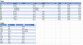
You can also debug one step at a time (using your worksheet posted in the image in Post #12), in B4 by slowly building up your formula by testing each of these sub subsections
(no guarantee this is typo free - but I hope you understand what I'm asking you to do):
1. Match($A4,$H$:$H$29,0) drag it down to confirm you're getting matches, if you're not then the data has some non printing characters.
2. Match("401L",$I$4:$I$I29,0), drag, confirm you have matches.
3. IF(B$3="Loan ID 1","401L","401L2"), drag, confirm, if no match then B3 has some non printing characters in it, retype "Loan ID 1" into the B3, see if it matches.
4. Match(IF(B$3="Loan ID 1","401L","401L2"),$I$4:$I$I29,0), drag, confirm you get some appropriate hits (you may get 401L2 numbers if it is not correct).
5. Match($A4&IF(B$3="Loan ID 1","401L","401L2"),$H$4:$H$29&$I$4:$I$29,0), drag, confirm you get appropriate hits.
6. INDEX($K$4:$K$29,Match($A4&IF(B$3="Loan ID 1","401L","401L2"),$H$4:$H$29&$I$4:$I$29,0),0), drag, confirm
7. IFERROR(INDEX($K$4:$K$29,Match($A4&IF(B$3="Loan ID 1","401L","401L2"),$H$4:$H$29&$I$4:$I$29,0),0),""), drag, confirm
8. Copy to column D, drag confirm.